Phreeqc Program Introduction,Using Phreeqc&Evaporation and Homogeneous Redox Reactions as a application
Introduciton
PHREEQC Version 3 is a computer program written in the C++ programming language that is designed to perform a wide variety of aqueous geochemical calculations. PHREEQC implements several types of aqueous models including two ion-association aqueous models.
Version 3.0--Documentation of all features, including high pressure calculations, charting (Windows), Pitzer and SIT activity-coefficient models, CD-MUSIC surface complexation, and isotope capabilities. Updated PhreeqcI. Additional methods for IPhreeqc modules.
PhreeqcRM--Reaction module for reactive-transport simulators. Based on IPhreeqc, allows access to all PHREEQC reaction capabilities. Contains methods for initial and boundary conditions, running reactions on all model cells, transfer of data to and from the module, and parallelization by MPI or OpenMP.
Using Phreeqc:
You know run capability of Notepad++!!!In this point,We will use this capability for phreeqc...You must download phreeqc3.installer executable application for this aim.And next,selecting executable application with run->run... steps.We will see phreeqc option related for run submenu of notepad++ after insallation steps;

Evaporation and Homogeneous Redox Reactions as a application:
I realised a save as evaporation.dat after input via newpage of program code related;
 |
| Input Dataset |
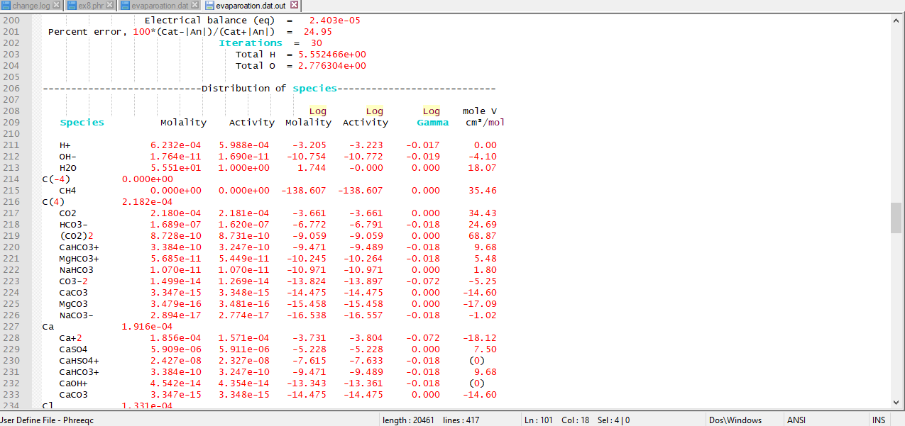
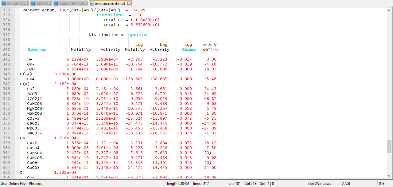
Next,compilation of program on redframe produced conclusions summaried with evaporation.dat.out format;
illustration of results after simulations Add Notes.Evaporation is accomplished by removing water from the chemical system. Water can be removed by two methods: (1) water can be specified as an irreversible reactant with a negative reaction coefficient in the REACTION keyword input, or (2) "H2O" can be specified as the alternative reaction in EQUILIBRIUM_PHASES keyword input, in which case, water is removed or added to the aqueous phase to attain a specified saturation index for a pure phase. This example uses the first method, the REACTION keyword data block is used to simulate concentration of rain water by approximately 20 fold by removing 95 percent of the water. The resulting solution contains only about 0.05 kg of water. In a subsequent simulation, the MIX keyword is used to generate a solution that has the same concentrations as the evaporated solution, but has a total of mass of water of approximately 1 kg.The first simulation input dataset contains four keywords: (1) TITLE is used to specify a description of the simulation to be included in the output file, (2) SOLUTION is used to define the composition of rain water from central Oklahoma, (3) REACTION is used to specify the amount of water, in moles, to be removed from the aqueous phase, and (4) SAVE is used to store the result of the reaction calculation as solution number 2.
All solutions defined by SOLUTION input are scaled to have exactly 1 kg (approximately 55.5 mol) of water. To concentrate the solution by 20 fold, it is necessary to remove approximately 52.8 mol of water (55.5 x 0.95).
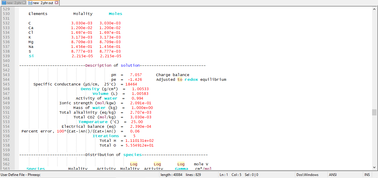
The second simulation uses MIX to multiply by 20 the number of moles of all elements in the solution, including hydrogen and oxygen. This procedure effectively increases the total mass (or volume) of the aqueous phase, but maintains the same concentrations. The resulting solution is stored in solution 3 with the SAVE keyword. Solution 3 will have the same concentrations as solution 2 (from the previous simulation) but will have a mass of water of approximately 1 kg.
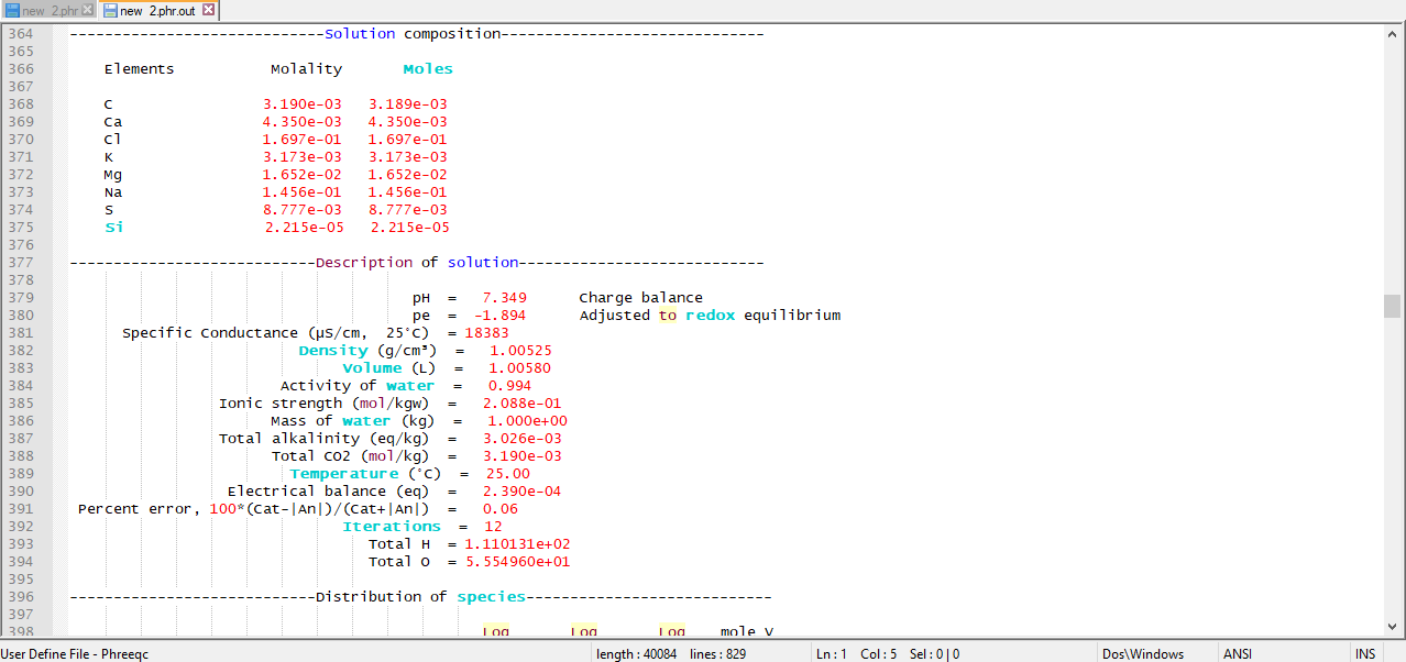
Selected results of the simulation are presented in table 10. The concentration factor of 20 is reasonable in terms of a water balance for the process of evapotranspiration in central Oklahoma (Parkhurst, Christenson, and Breit, 1993). However, the PHREEQC evaporation modeling assumes that evapotranspiration has no affect on the ion ratios. This assumption has not been verified and may not be correct. After evaporation, the simulated solution composition is still undersaturated with respect to calcite, dolomite, and gypsum. As expected, the mass of water decreases from 1 kg in rain water (solution 1) to approximately 0.05 kg in solution 2 after water was removed by the reaction. In general, the amount of water remaining after the reaction is approximate because water may be consumed or produced by homogeneous hydrolysis reactions, surface complexation reactions, and dissolution and precipitation of pure phases. The number of moles of chloride (mmol) was unaffected by the removal of water; however, the concentration of chloride (mmol/kg water) increased because the amount of water decreased. The mixing simulation increased the mass of water and the number of moles of chloride by a factor of 20. Thus, the number of moles of chloride increased, but the concentration is the same before (solution 2) and after the mixing simulation (solution 3) because of the increased mass of water.
An important point about homogeneous redox reactions is illustrated in the results of these simulations . Reaction calculations always produce redox equilibrium. The rain water analysis contained data for both ammonium and nitrate, but none for dissolved nitrogen. Although nitrate and ammonium should not coexist at thermodynamic equilibrium, the speciation calculation allows redox disequilibria and the concentrations of the nitrogen species are defined only by the input data. In the reaction (evaporation) step, redox equilibrium is attained for the aqueous phase, which caused ammonium to be oxidized and nitrate to be reduced, generating dissolved nitrogen. The equilibrium solution (solution 2) contains nitrate and dissolved nitrogen, but virtually no ammonium (illustration of results after simulations). This redox equilibration will occur in the reaction calculation because of the inherent redox disequilibrium in the definition of the rain water composition. Nitrogen redox reactions would have occurred even if the REACTION keyword had specified that no water was to be removed.
Updates:
Mixing Application
This example demonstrates the capabilities of PHREEQC to perform a series of geochemical simulations, with the final simulations relying on results from previous simulations within the same run. The example investigates diagenetic reactions that may occur in zones where seawater mixes with carbonate ground water. The example is divided into five simulations, labeled A through E in Example 3. (A) Carbonate ground water is defined by equilibrating pure water with calcite at a
of 10-2.0 atm. (B) Seawater is defined using the major-ion data given in table 2. (C) The two solutions are mixed together in the proportions 30 percent seawater and 70 percent ground water. (D) The mixture is equilibrated with calcite and dolomite. Finally, (E) the mixture is equilibrated with calcite only to simulate slow reaction kinetics of dolomite.


TITLE Example 3, part A--Calcite equilibrium at log Pco2 = -2.0 and 25C.
SOLUTION 1  Pure water
        pH      7.0
        temp    25.0
EQUILIBRIUM_PHASES
        CO2(g)          -2.0
        Calcite         0.0
SAVE solution 1
END
TITLE Example 3, part B--Definition of seawater.
SOLUTION 2  Seawater
        units   ppm
        pH      8.22
        pe      8.451
        density 1.023
        temp    25.0
        Ca              412.3
        Mg              1291.8
        Na              10768.0
        K               399.1
        Si              4.28
        Cl              19353.0
        Alkalinity      141.682 as HCO3
        S(6)            2712.0
END
TITLE Example 3, part C--Mix 70% ground water, 30% seawater.
MIX 1
        1      0.7
        2      0.3
SAVE solution   3
END
TITLE Example 3, part D--Equilibrate mixture with calcite and dolomite.
EQUILIBRIUM_PHASES 1
        Calcite         0.0
        Dolomite        0.0
USE solution 3
END
TITLE Example 3, part E--Equilibrate mixture with calcite only.
EQUILIBRIUM_PHASES 2
        Calcite         0.0
USE solution 3
END
A summary of compilation conclusions;


The input for part A (Example 3) consists of the definition of pure water with SOLUTION input, and the definition of a pure-phase assemblage with EQUILIBRIUM_PHASES input. In the definition of the phases, only a saturation index was given for each phase. Because it was not entered, the amount of each phase defaults to 10.0 mol, which is essentially an unlimited supply for most phases. The reaction is implicitly defined to be the equilibration of the first solution defined in this simulation with the first pure-phase assemblage defined in the simulation. (Explicit definition of reaction entities is done with the USE keyword.) The SAVE keyword instructs the program to save the solution following the final (and only in this example) reaction step as solution number 1. Thus, when the simulation begins, solution number 1 is pure water. After the reaction calculations for the simulation are completed, the composition of the water that is in equilibrium with calcite and CO2 replaces pure water as solution 1.Part B defines the composition of seawater, which is stored as solution number 2. Part C mixes ground water, solution 1, with seawater, solution 2, in a closed system in which  is calculated, not specified. The MIX keyword is used to define the solutions and mixing fractions. The SAVE keyword causes the mixture to be saved as solution number 3. The MIX keyword allows the mixing of an unlimited number of solutions in whatever fractions are specified. The fractions need not sum to 1.0. If the fractions were 7.0 and 3.0 instead of 0.7 and 0.3, the mass of water in the mixture would be approximately 10 kg instead of approximately 1 kg, but the concentrations in the mixture would be the same as in this example. However, during subsequent reactions it would take approximately 10 times more mole transfer to equilibrate with the phases, that is, to produce the same concentrations as in this example.
Part D equilibrates the mixture with calcite and dolomite. The USE keyword specifies that solution number 3, which is the mixture from part C, is to be the solution with which the phases will equilibrate. By defining the phase assemblage with "EQUILIBRIUM_PHASES 1", the phase assemblage replaces the previous assemblage number 1 that was defined in part A. Part E performs a similar calculation to part D, but uses phase assemblage 2, which does not contain dolomite as a reactant.

Conclusions
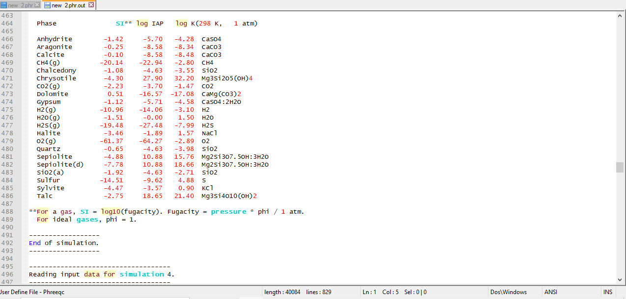
Selected results from the output for example 3 are presented in Conclusions. The ground water produced by part A is in equilibrium with calcite and has a log  of -2.0, as specified by the input. The moles of CO2 in the phase assemblage decreased by about 2.0 mmol, which means that about 2.0 mmol dissolved into solution. Likewise, about 1.6 mmol of calcite dissolved. Part B defined seawater, which is calculated to have slightly greater than atmospheric carbon dioxide (-3.38 compared to about -3.5), and is supersaturated with calcite (saturation index 0.76) and dolomite (2.40). No mole transfer was allowed for part B. Part C performed the mixing with no additional reactions. The resulting log
  is -2.23, calcite is undersaturated and dolomite is supersaturated. The saturation indices indicate that thermodynamically, dolomitization should occur, that is calcite should dissolve and dolomite should precipitate. Part D calculates the amounts of calcite and dolomite that should react. To produce equilibrium 15.7 mmol of calcite should dissolve and 7.9 mmol of dolomite should precipitate. Dolomitization is not observed to occur in present-day mixing zone environments, even though dolomite is the thermodynamically stable phase. The lack of significant dolomitization is due to the slow reaction kinetics of dolomite formation. Therefore, part E simulates what would happen if dolomite does not precipitate. If dolomite does not precipitate, only a very small amount of calcite dissolves (0.04 mmol) for this mixing ratio.
Application of Equilibration with Pure Phases
This example determines the solubility of the most stable phase, gypsum or anhydrite, over a range of temperatures. The input dataset is bottom part . Only the pH and temperature are used to define the pure water solution. Default units are millimolal, but no concentrations are specified. By default, pe is 4.0, the default redox calculation uses pe, and the density is 1.0 (not needed because no concentrations are "per liter"). All phases that are allowed to react to a specified saturation index during the reaction calculation are listed in EQUILIBRIUM_PHASES, whether they are initially present or not. The input data include the name of the phase (previously defined through PHASES input in the database or input file), the specified saturation index, and the amount of the phase present, in moles. If a phase is not present initially, it is given 0.0 mol in the pure-phase assemblage. In this example, gypsum and anhydrite are allowed to react to equilibrium (saturation index equal to 0.0), and the initial phase assemblage has 1 mol of each mineral. Each mineral will react either to equilibrium or until it is exhausted in the assemblage. In most cases, 1 mol of a phase is sufficient to reach equilibrium
TITLE Example Temperature dependence of solubility of gypsum and anhydrite
SOLUTION 1 Pure water
pH 7.0
temp 25.0
EQUILIBRIUM_PHASES 1
Gypsum 0.0 1.0
Anhydrite 0.0 1.0
REACTION_TEMPERATURE 1
25.0 75.0 in 51 steps
SELECTED_OUTPUT
-file gypsum.sel
-temperature
-si anhydrite gypsum
USER_GRAPH 1 Example 2
-headings Temperature Gypsum Anhydrite
-chart_title "Gypsum-Anhydrite Stability"
-axis_scale x_axis 25 75 5 0
-axis_scale y_axis auto 0.05 0.1
-axis_titles "Temperature, in degrees celsius" "Saturation index"
-initial_solutions false
-start
10 graph_x TC
20 graph_y SI("Gypsum") SI("Anhydrite")
-end
END
A set of 51 temperatures is specified in the REACTION_TEMPERATURE data block. The input data specify that for every degree of temperature, beginning at 25oC and ending at 75oC, the phases defined by EQUILIBRIUM_PHASES (gypsum and anhydrite) will react to attain equilibrium, if possible, or until both phases are completely dissolved. Finally, SELECTED_OUTPUT is used to write the saturation indices for gypsum and anhydrite to file related after each calculation. This file was then used to generate figure 1.

Figure 1_Saturation indices of Gypsum and Anhydrite in solutions that have equilibrated with the more stable of the two phases over the tempreature range 25 to 75 degree Celsius.


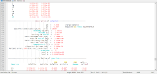
The results of the initial solution calculation and the first reaction step are shown in Figure 2. The distribution of species for pure water is shown under the heading "Beginning of initial solution calculations". The equilibration of the system with the given amounts of gypsum and anhydrite at 25oC is the first reaction step, which is displayed after the heading "Beginning of reaction calculations". Immediately following this heading, the reaction step is identified, followed by a list of the identity of the keyword data used in the calculation. In this example, the solution composition stored as number 1, the pure-phase assemblage stored as number 1, and the reaction temperatures stored as number 1 are used in the calculation. Conceptually, the solution and the pure phases are put together in a beaker, which is regulated to 25oC, and allowed to react to system equilibrium.
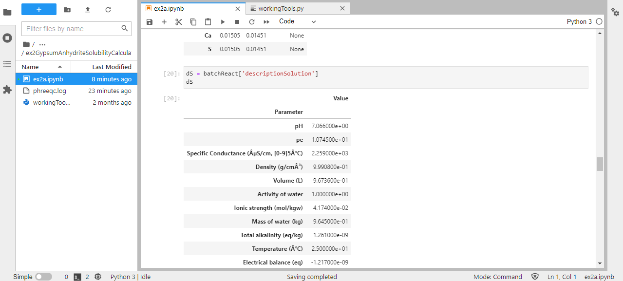
Under the subheading "Phase assemblage", the saturation indices and amounts of each of the phases defined by EQUILIBRIUM_PHASES are listed. In the first reaction step, the final phase assemblage contains no anhydrite, which is undersaturated with respect to the solution (saturation index equals -0.22), and 1.985 mol of gypsum, which is in equilibrium with the solution (saturation index equals 0.0). All of the anhydrite has dissolved and most of the calcium and sulfate have reprecipitated as gypsum. The "Solution composition" indicates that 15.67 mmol/kg water of calcium and sulfate remain in solution, which defines the solubility of gypsum in pure water. However, the total number of moles of each constituent in the aqueous phase is only 15.11 because the mass of water is only 0.9645 kg ("Description of solution"). In precipitating gypsum (CaSO4.2H2O), water has been removed from solution. Thus, the mass of solvent water is not constant in reaction calculations as it was in PHREEQE; reactions and waters of hydration in dissolving and precipitating phases may increase or decrease the mass of solvent water.
The saturation indices for all of the reaction steps are plotted in figure 1. In each step, pure water was reacted with the phases at a different temperature (the reactions are not cumulative). The default database for PHREEQC indicates that gypsum is the stable phase (saturation index equals 0.0) at temperatures below about 57oC; above this temperature, anhydrite is the stable phase.
------------------
Reading data base.
------------------
        SOLUTION_SPECIES
        SOLUTION_MASTER_SPECIES
        PHASES
        EXCHANGE_MASTER_SPECIES
        EXCHANGE_SPECIES
        SURFACE_MASTER_SPECIES
        SURFACE_SPECIES
        END
------------------------------------
Reading input data for simulation 1.
------------------------------------
        TITLE
        Example 2.--Temperature dependence of solubility
                    of gypsum and anhydrite
        SOLUTION 1 Pure water
                pH      7.0
                temp    25.0
        EQUILIBRIUM_PHASES 1
                Gypsum          0.0     1.0
                Anhydrite       0.0     1.0
        REACTION_TEMPERATURE 1
                25.0 75.0 in 51 steps
        SELECTED_OUTPUT
                file   ex2.pun
                si     anhydrite  gypsum
        END
-----
TITLE
-----
Example 2.--Temperature dependence of solubility
            of gypsum and anhydrite
-------------------------------------------
Beginning of initial solution calculations.
-------------------------------------------
Initial solution 1.     Pure water
-----------------------------Solution composition------------------------------

        Elements           Molality       Moles
        Pure water
----------------------------Description of solution----------------------------
                             pH  =   7.000
                             pe  =   4.000
              Activity of water  =   1.000
                 Ionic strength  =   1.001e-07
             Mass of water (kg)  =   1.000e+00
       Total alkalinity (eq/kg)  =   1.082e-10
          Total carbon (mol/kg)  =   0.000e+00
             Total CO2 (mol/kg)  =   0.000e+00
            Temperature (deg C)  =  25.000
        Electrical balance (eq)  =  -1.082e-10
                     Iterations  =   2
                        Total H  = 1.110124e+02
                        Total O  = 5.550622e+01

----------------------------Distribution of species----------------------------
                                                   Log       Log         Log
        Species            Molality    Activity  Molality  Activity     Gamma

        OH-               1.001e-07   1.001e-07    -6.999    -7.000     0.000
        H+                1.000e-07   1.000e-07    -7.000    -7.000     0.000
        H2O               5.551e+01   1.000e+00     0.000     0.000     0.000
H(0)             1.416e-25
        H2                7.079e-26   7.079e-26   -25.150   -25.150     0.000
O(0)             0.000e+00
        O2                0.000e+00   0.000e+00   -42.080   -42.080     0.000

------------------------------Saturation indices-------------------------------
        Phase               SI log IAP  log KT

        H2(g)           -22.00  -22.00    0.00  H2
        O2(g)           -39.12   44.00   83.12  O2
-----------------------------------
Beginning of reaction calculations.
-----------------------------------

Reaction step 1.

Using solution 1.       Pure water

Using pure phase assemblage 1.

Using temperature 1.

             25.00 is current temperature.
-------------------------------Phase assemblage--------------------------------
                                                     Moles in assemblage
        Phase               SI log IAP  log KT    Initial      Final      Delta
        Anhydrite        -0.22   -4.58   -4.36  1.000e+00            -1.000e+00
        Gypsum            0.00   -4.58   -4.58  1.000e+00  1.985e+00  9.849e-01
-----------------------------Solution composition------------------------------
        Elements           Molality       Moles
        Ca                1.567e-02   1.511e-02
        S                 1.567e-02   1.511e-02

----------------------------Description of solution----------------------------
                             pH  =   7.062      Charge balance
                             pe  =   4.111      Adjusted to redox equilibrium
              Activity of water  =   1.000
                 Ionic strength  =   4.190e-02
             Mass of water (kg)  =   9.645e-01
       Total alkalinity (eq/kg)  =   1.122e-10
          Total carbon (mol/kg)  =   0.000e+00
             Total CO2 (mol/kg)  =   0.000e+00
            Temperature (deg C)  =  25.000
        Electrical balance (eq)  =  -1.082e-10
                     Iterations  =  13
                        Total H  = 1.070729e+02
                        Total O  = 5.359687e+01

----------------------------Distribution of species----------------------------
                                                   Log       Log         Log
        Species            Molality    Activity  Molality  Activity     Gamma

        OH-               1.403e-07   1.155e-07    -6.853    -6.938    -0.085
        H+                1.007e-07   8.666e-08    -6.997    -7.062    -0.065
        H2O               5.551e+01   9.996e-01     0.000     0.000     0.000
Ca               1.567e-02
        Ca+2              1.047e-02   5.176e-03    -1.980    -2.286    -0.306
        CaSO4             5.191e-03   5.242e-03    -2.285    -2.281     0.004
        CaOH+             1.192e-08   9.909e-09    -7.924    -8.004    -0.080
H(0)             6.322e-26
        H2                3.161e-26   3.192e-26   -25.500   -25.496     0.004
O(0)             0.000e+00
        O2                0.000e+00   0.000e+00   -41.393   -41.388     0.004
S(-2)            0.000e+00
        HS-               0.000e+00   0.000e+00   -65.005   -65.090    -0.085
        H2S               0.000e+00   0.000e+00   -65.162   -65.158     0.004
        S-2               0.000e+00   0.000e+00   -70.633   -70.946    -0.313
S(6)             1.567e-02
        SO4-2             1.047e-02   5.075e-03    -1.980    -2.295    -0.315
        CaSO4             5.191e-03   5.242e-03    -2.285    -2.281     0.004
        HSO4-             5.145e-08   4.276e-08    -7.289    -7.369    -0.080

------------------------------Saturation indices-------------------------------
        Phase               SI log IAP  log KT

        Anhydrite        -0.22   -4.58   -4.36  CaSO4
        Gypsum            0.00   -4.58   -4.58  CaSO4:2H2O
        H2(g)           -22.35  -22.35    0.00  H2
        H2S(g)          -64.16 -105.80  -41.64  H2S
        O2(g)           -38.43   44.69   83.12  O2
        Sulfur          -47.69  -83.46  -35.76  S


Input Data:https://hatarilabs.com/ih-en/gypsum-and-anhydrite-solubility-calculation-with-phreeqc-and-python-tutorial

Yorumlar
Yorum Gönder