Kayıtlar

Ekim, 2018 tarihine ait yayınlar gösteriliyor

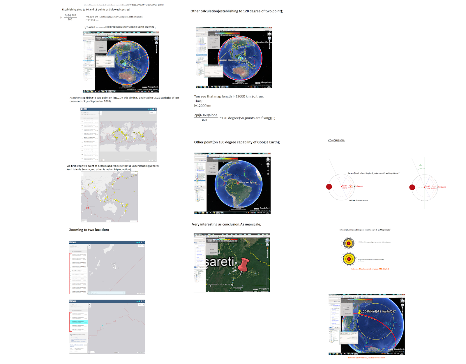
Best Hazardous Regions of World by Swarm&Triple Juction relation

Resim
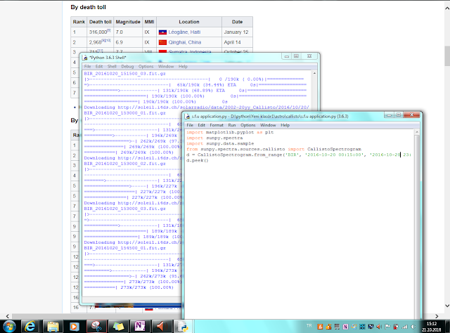
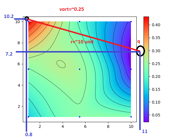
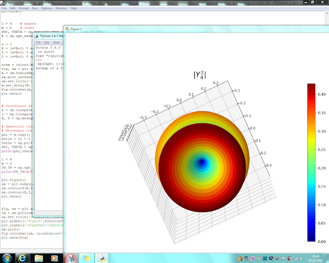
Sulawesi Event that great experiment for numeric studies... I realised some test calculations that opening to such a part  by conclusions is a requirement for various sub-chapter; I identified to swarm via a querying for last one month on USGS data;         Next,other steps on Lenght;              Conclusion: East Kalimantan Coasts     ----------------------------------------------------------------------------------   Via a querying as monthly for October 2012;                 Conclusion: New Zealand-North Island Region

#A mehodology for source mechanism studies

Resim
I shared a information; https://plus.google.com/u/0/109215510128907332215/posts/C3WNixicgV8 This time that methodology of source mechanism via applying to Earth Model to this model will understand... Thus,I analysed for Sulawesi Event that on USGS statistics of last onemonth(Conclusions as a whole are Poster Presentation);

Callisto Spectrogram Application of Sunpy

Resim
Earthquake researchings among Callisto Spectrogram applications that expressing as quite popular... Where,conclusions for a test of s.f.u. application on date range of Sunpy are considering; import matplotlib.pyplot as plt import sunpy.spectra import sunpy.data.sample from sunpy.spectra.sources.callisto import CallistoSpectrogram d = CallistoSpectrogram.from_range('BIR', '2016-10-20 00:15:00', '2016-10-20 23:45:00') d.peek() ------------------------------------------------- Official Page as actual following on Data Comparison Methodology ;                                 http://www.e-callisto.org/                                                                                                                                                                                                                                                                            Datapage for USGS Earthquake Cataloque ;                  

E Field Distribution Solution on Four Charge Model

Resim
import numpy as np import matplotlib.pyplot as plt from scipy.interpolate import griddata npts=200 xmin, xmax = 1, 10 ymin, ymax = 1, 10 x = np.array([1, 1, 1, 5.5, 5.5, 5.5, 10, 10, 10]) y = np.array([1, 5.5, 10, 1, 5.5, 10, 1, 5.5, 10]) #Voltage input z = np.array([23.78, 23.78, 20.45, 24.38, 18.55,               27.26, 5.24, 22.32, 5.53]) xi = np.linspace(xmin, xmax, npts) yi = np.linspace(ymin, ymax, npts) zi = griddata((x, y), z, (xi[None,:], yi[:,None]), method='cubic') plt.contour(xi, yi, zi, 15, linewidths=0.5, colors='k') plt.pcolormesh(xi, yi, zi, cmap=plt.get_cmap('rainbow')) plt.colorbar() plt.scatter(x, y, marker='o', c='b', s=5, zorder=10) plt.show() plt.contourf(xi,yi,zi,15,cmap=plt.cm.jet) plt.show() #Input of Mean Voltage and distance for two-charge condition #where,effect force on other charge on q=1 condition is calculating vort=0.55 r=7.07 f=vort/r print(f) #Next,F=k(q.aq)/(r^2) formulation that calculates a coefficin

Linguistic Chapters

Resim
What is "Wild English" Concept? "Wild English" concept that I evaluate using by French Nation.By Actual English,expressed English shape at Britain Island of ancient times that as incomprehensible by linguistics is explaining. On Actual English,due to chapters as inverse structure of world syntax by French with taking place of French Words as very dominant thus particular perceptions about saying causes by French Nation of "Wild English" is understanding. Europe Region based on Latin Alphabet  Distinction as Latin&North type is recognising.Thus,a base grouping between English,German Languages and Spanish,French,Italian  can express.A explaining as list;

E Field Distribution Solution on Three Charge Model

Resim
This time,a approach for three charge model of same charges import numpy as np import matplotlib.pyplot as plt from scipy.interpolate import griddata npts=200 xmin, xmax = 1, 10 ymin, ymax = 1, 10 x = np.array([1, 1, 1, 5.5, 5.5, 5.5, 10, 10, 10]) y = np.array([1, 5.5, 10, 1, 5.5, 10, 1, 5.5, 10]) #Voltage input z = np.array([0.68, 0.78, 0.435, 0.638, 0.555,               0.263, 0.234, 0.532, 0.553]) xi = np.linspace(xmin, xmax, npts) yi = np.linspace(ymin, ymax, npts) zi = griddata((x, y), z, (xi[None,:], yi[:,None]), method='cubic') plt.contour(xi, yi, zi, 15, linewidths=0.5, colors='k') plt.pcolormesh(xi, yi, zi, cmap=plt.get_cmap('rainbow')) plt.colorbar() plt.scatter(x, y, marker='o', c='b', s=5, zorder=10) plt.show() plt.contourf(xi,yi,zi,15,cmap=plt.cm.jet) plt.show() #Input of Mean Voltage and distance for two-charge condition #where,effect force on other charge on q=1 condition is calculating vort=0.55 r=7.07 f=vort/r print(f)

E Field Distribution Solution on Two Charge Model

Resim
Established studies for understanding to Electric Field  among maybe best important points on Applied Geophysics field can express...This application thus,explaining a solution on two-charge model; import numpy as np import matplotlib.pyplot as plt from scipy.interpolate import griddata npts=200 xmin, xmax = 1, 10 ymin, ymax = 1, 10 x = np.array([1, 1, 1, 5.5, 5.5, 5.5, 10, 10, 10]) y = np.array([1, 5.5, 10, 1, 5.5, 10, 1, 5.5, 10]) #Voltage input z = np.array([0.148, 0.238, 0.435, 0.238, 0.255,               0.203, 0.234, 0.032, 0.053]) xi = np.linspace(xmin, xmax, npts) yi = np.linspace(ymin, ymax, npts) zi = griddata((x, y), z, (xi[None,:], yi[:,None]), method='cubic') plt.contour(xi, yi, zi, 15, linewidths=0.5, colors='k') plt.pcolormesh(xi, yi, zi, cmap=plt.get_cmap('rainbow')) plt.colorbar() plt.scatter(x, y, marker='o', c='b', s=5, zorder=10) plt.show() plt.contourf(xi,yi,zi,15,cmap=plt.cm.jet) plt.show() #Input of Mean Volt

a representation of the spherical harmonic as a heatmap of a field with a Mollweide projection

Resim
Modelling Studies for Geophysicists quite important.Thus,A Globe Modelling Example which presenting on python programming language.Chapter as Summary; expressing as a representation of the spherical harmonic as a heatmap of a field with a Mollweide projection from __future__ import division import scipy as sci import scipy.special as sp import numpy as np import matplotlib import matplotlib.pyplot as plt from mpl_toolkits.mplot3d import Axes3D from matplotlib import cm, colors #Example to calculate Y_4^2 l = 4 m = 2 theta, phi = 0.6, 0.75    # Some arbitrary values of angles in radians Y42 = sp.sph_harm(m, l, phi, theta) z = np.cos(theta) P42 = sp.lpmv(m,l,z) f = sci.math.factorial K_norm = np.sqrt((2*l+1)/(4 * np.pi) * f(l-m)/f(l+m)) K_norm * P42* np.exp(m*phi*1j) == Y42 def dotprod(f,g):     #Scipy does not directly integrates complex functions.     #You have to break them down into two integrals of the real and imaginary part     integrand_r = lambda theta

Megalithic Structures

Resim
Understanding to Difference Unfortunately,I see "Big Information Pollution"about Megaliths.Firstly,I must say that a Megalith expression for everystructure isn't true!!!But,"Megalithic Structure "expression is true.As clear,a scheme;   about Role of "Megalithic Structures" Having to role for understanding to realised Geologic Processes in actual time at this cultural environments with understanding to Antropogenic Development based on Prehistoric Culture Menhir Structure Menhir shortly that expressing as relative small rockmass or angular string rockmasses on scheme .Not only taking place among quite base points for implications of lost settlements on especially archaeologic concept also important with role playing as direct/indirect to/of other vocational disciplines.Thus,Menhir Scholarship evaluating as a field as quite popular.In this blog,I will work to compiling to some conclusions about Menhir Structures at World on time