Signal Processing with Python
Big part of methods in Geophysics are base of signal processing.
Amplitude,Phase,Frequency informations for this type measurements are producing.But,requirement to this type data for some measurment types is not;
import numpy as np
from scipy.interpolate import Rbf
import matplotlib.pyplot as plt
import matplotlib.cm as cm
#x,y coordinates
x = [25,25,25,25,25,25,25,50,50,50,50,50,50,50,75,75,75,75,75,75,75,100,100,100,100,100,100,100,125,125,125,125,125,125,125,150,150,150,150,150,150,150,175,175,175,175,175,175,175]
y = [25,50,75,100,125,150,175,25,50,75,100,125,150,175,25,50,75,100,125,150,175,25,50,75,100,125,150,175,25,50,75,100,125,150,175,25,50,75,100,125,150,175,25,50,75,100,125,150,175]
#Potential by Reference Electrode of Platin Electrode in Soil
sp = [400,350,200,400,-150,150,-100,-150,-155,-4.5,-13,14,15,-30,-50,-30,100,-20,20,-300,-300,-25,-270,-200,-220,-200,-300,-330,-320,-120,-540,-400,-300,-120,-100,100,300,-100,200,100,150,100,150,-200,-300,-120,-110,-400,-300]
#Potential of Reference Electrode by Standard Hydrogen Electrode
eref=[316,316,316,316,316,316,316,316,316,316,316,316,316,316,316,316,316,316,316,316,316,316,316,316,316,316,316,316,316,316,316,316,316,316,316,316,316,316,316,316,316,316,316,316,316,316,316,316,316]
ph=[5,7,7.1,7.2,8,6.2,6.7,7.2,6,7.2,6.4,7.1,7.4,8.3,8.1,8.0,7.6,7.4,7.1,6.9,7,6.4,6.0,6.2,6.5,7.1,7.3,6.5,7.1,7.3,7.3,7.2,5.5,5.6,6.1,6.3,6.6,6.8,7.0,7,7.1,7.3,6.9,6.7,6,7,6.6,6.3,6.1]
sp=np.asarray(sp)
eref=np.asarray(eref)
ph=np.asarray(ph)
red=sp+eref-60*(ph-7)
#200x200 dimension field production
ti = np.linspace(0, 200.0, 200)
XI, YI = np.meshgrid(ti, ti)
#selecting to kriging function type(linear,multiquadric,inverse,gaussian,cubic,quintic,thin_plate)
rbf = Rbf(x, y, red, function='inverse')
ZI = rbf(XI, YI)
#Distribution as Conclusion
plt.subplot(1, 1, 1)
plt.pcolor(XI, YI, ZI,cmap=cm.jet)
plt.scatter(x, y, 1, red,cmap=cm.jet)
plt.title('Soil Redox Potential Distribution ')
plt.xlim(0, 200)
plt.ylim(0, 200)
plt.colorbar()
plt.show()

import scipy.io.wavfile
from pydub import AudioSegment
import pydub
#a temp folder for downloads
temp_folder="/Users/Geo/Desktop/"
#spotify mp3 sample file
web_file="https://p.scdn.co/mp3-preview/0ba9d38f5d1ad30f0e31fc8ee80c1bebf0345a0c"
#download file
urllib.request.urlretrieve(web_file,temp_folder+"file.mp3")
#read mp3 file
AudioSegment.converter = "/ffmpeg/bin/ffmpeg"
mp3 = pydub.AudioSegment.from_mp3(temp_folder+"file.mp3")
#convert to wav
mp3.export(temp_folder+"file.wav", format="wav")
#read wav file
rate,audData=scipy.io.wavfile.read(temp_folder+"file.wav")
#the sample rate is the number of bits of information recorded per second
print(rate)
print(audData)
#wav bit type the amount of information recorded in each bit often 8, 16 or 32 bit
audData.dtype
#wav length
audData.shape[0] / rate
#wav number of channels mono/stereo
audData.shape[1]
#if stereo grab both channels
channel1=audData[:,0] #left
channel2=audData[:,1] #right
np.sum(channel1.astype(float)**2)
#this can be infinite and depends on the length of the music of the loudness often talk about power
#power - energy per unit of time
1.0/(2*(channel1.size)+1)*np.sum(channel1.astype(float)**2)/rate
#save a file at half and double speed
scipy.io.wavfile.write(temp_folder+"file2.wav", rate/2, audData)
scipy.io.wavfile.write(temp_folder+"file2.wav", rate*2, audData)
#save a single channel
scipy.io.wavfile.write(temp_folder+"file2.wav", rate, channel1)
#averaging the channels damages the music
mono=np.sum(audData.astype(float), axis=1)/2
scipy.io.wavfile.write(temp_folder+"file2.wav", rate, mono)
#plot amplitude (or loudness) over time
plt.figure(1)
plt.subplot(211)
plt.plot(time, channel1, linewidth=0.02, alpha=0.7, color='#ff7f00')
plt.xlabel('Time (s)')
plt.ylabel('Amplitude')
plt.subplot(212)
plt.plot(time, channel2, linewidth=0.02, alpha=0.7, color='#ff7f00')
plt.xlabel('Time (s)')
plt.ylabel('Amplitude')
plt.savefig(temp_folder+'ampiltude.png', bbox_inches='tight')
#a fourier transform breaks the sound wave into series of waves that make up the main sound wave
#each of these waves will have its own amplitude (volume) and frequency. The frequency is the length over which the wave repeats itself. this is known as the pitch of the sound
from numpy import fft as fft
fourier=fft.fft(channel1)
plt.figure(1, figsize=(8,6))
plt.plot(fourier, color='#ff7f00')
plt.xlabel('k')
plt.ylabel('Amplitude')
plt.savefig(temp_folder+'fft.png', bbox_inches='tight')
#the fourier is symetrical due to the real and imaginary soultion. only interested in first real solution
n = len(channel1)
fourier = fourier[0:(n/2)]
# scale by the number of points so that the magnitude does not depend on the length
fourier = fourier / float(n)
#calculate the frequency at each point in Hz
freqArray = np.arange(0, (n/2), 1.0) * (rate*1.0/n);
plt.figure(1, figsize=(8,6))
plt.plot(freqArray/1000, 10*np.log10(fourier), color='#ff7f00', linewidth=0.02)
plt.xlabel('Frequency (kHz)')
plt.ylabel('Power (dB)')
plt.savefig(temp_folder+'frequencies.png', bbox_inches='tight')
#plot spectogram
#the function calculates many fft's over NFFT sized blocks of data
#increasing NFFT gives you a more detail across the spectrum range but decreases the samples per second
#the sampling rate used determines the frequency range seen always 0 to rate/2
plt.figure(2, figsize=(8,6))
plt.subplot(211)
Pxx, freqs, bins, im = plt.specgram(channel1, Fs=rate, NFFT=1024, cmap=plt.get_cmap('autumn_r'))
cbar=plt.colorbar(im)
plt.xlabel('Time (s)')
plt.ylabel('Frequency (Hz)')
cbar.set_label('Intensity dB')
plt.subplot(212)
Pxx, freqs, bins, im = plt.specgram(channel2, Fs=rate, NFFT=1024, cmap=plt.get_cmap('autumn_r'))
cbar=plt.colorbar(im)
plt.xlabel('Time (s)')
plt.ylabel('Frequency (Hz)')
cbar.set_label('Intensity (dB)')
#plt.show()
plt.savefig(temp_folder+'spectogram.png', bbox_inches='tight')
#Larger Window Size value increases frequency resolution
#Smaller Window Size value increases time resolution
#Specify a Frequency Range to be calculated for using the Goertzel function
#Specify which axis to put frequency
Pxx, freqs, timebins, im = plt.specgram(channel2, Fs=rate, NFFT=1024, noverlap=0, cmap=plt.get_cmap('autumn_r'))
channel1.shape
Pxx.shape
freqs.shape
timebins.shape
np.min(freqs)
np.max(freqs)
np.min(timebins)
np.max(timebins)
np.where(freqs==10034.47265625)
MHZ10=Pxx[233,:]
plt.figure(figsize=(8,6))
plt.plot(timebins, MHZ10, color='#ff7f00')
plt.savefig(temp_folder+'MHZ10.png', bbox_inches='tight')

Thus,I produced to most good condition for Program
TEST_2
#required libraries
import urllib.request
import scipy.io.wavfile
from pydub import AudioSegment
import pydub
#a temp folder for downloads
temp_folder="/Users/Geo/Desktop/"
#spotify mp3 sample file
web_file="http://p.scdn.co/mp3-preview/35b4ce45af06203992a86fa729d17b1c1f93cac5"
#download file
urllib.request.urlretrieve(web_file,temp_folder+"file.mp3")
#read mp3 file
AudioSegment.converter = "/ffmpeg/bin/ffmpeg"
mp3 = pydub.AudioSegment.from_mp3(temp_folder+"file.mp3")
#convert to wav
mp3.export(temp_folder+"file.wav", format="wav")
#read wav file
rate,audData=scipy.io.wavfile.read(temp_folder+"file.wav")
#the sample rate is the number of bits of information recorded per second
print(rate)
print(audData)
#wav bit type the amount of information recorded in each bit often 8, 16 or 32 bit
audData.dtype
#wav length
audData.shape[0] / rate
#wav number of channels mono/stereo
audData.shape[1]
#if stereo grab both channels
channel1=audData[:,0] #left
channel2=audData[:,1] #right
import numpy as np
#Energy of music
np.sum(channel1.astype(float)**2)
#this can be infinite and depends on the length of the music of the loudness often talk about power
#power - energy per unit of time
1.0/(2*(channel1.size)+1)*np.sum(channel1.astype(float)**2)/rate
#save a single channel
scipy.io.wavfile.write(temp_folder+"file2.wav", rate, channel1)
#averaging the channels damages the music
mono=np.sum(audData.astype(float), axis=1)/2
scipy.io.wavfile.write(temp_folder+"file2.wav", rate, mono)
import matplotlib.pyplot as plt
time = np.arange(0, float(audData.shape[0]), 1) / rate
#plot amplitude (or loudness) over time
plt.figure(1)
plt.subplot(211)
plt.plot(time, channel1, linewidth=0.02, alpha=0.7, color='#ff7f00')
plt.xlabel('Time (s)')
plt.ylabel('Amplitude')
plt.subplot(212)
plt.plot(time, channel2, linewidth=0.02, alpha=0.7, color='#ff7f00')
plt.xlabel('Time (s)')
plt.ylabel('Amplitude')
plt.savefig(temp_folder+'ampiltude.png', bbox_inches='tight')
#Frequency (pitch) over time
#a fourier transform breaks the sound wave into series of waves that make up the main sound wave
#each of these waves will have its own amplitude (volume) and frequency. The frequency is the length over which the wave repeats itself. this is known as the pitch of the sound
from numpy import fft as fft
fourier=fft.fft(channel1)
plt.figure(1, figsize=(8,6))
plt.plot(fourier, color='#ff7f00')
plt.xlabel('k')
plt.ylabel('Amplitude')
plt.savefig(temp_folder+'fft.png', bbox_inches='tight')
#plot spectogram
#the function calculates many fft's over NFFT sized blocks of data
#increasing NFFT gives you a more detail across the spectrum range but decreases the samples per second
#the sampling rate used determines the frequency range seen always 0 to rate/2
plt.figure(2, figsize=(8,6))
plt.subplot(211)
Pxx, freqs, bins, im = plt.specgram(channel1, Fs=rate, NFFT=1024, cmap=plt.get_cmap('autumn_r'))
cbar=plt.colorbar(im)
plt.xlabel('Time (s)')
plt.ylabel('Frequency (Hz)')
cbar.set_label('Intensity dB')
plt.subplot(212)
Pxx, freqs, bins, im = plt.specgram(channel2, Fs=rate, NFFT=1024, cmap=plt.get_cmap('autumn_r'))
cbar=plt.colorbar(im)
plt.xlabel('Time (s)')
plt.ylabel('Frequency (Hz)')
cbar.set_label('Intensity (dB)')
plt.show()
plt.savefig(temp_folder+'spectogram.png', bbox_inches='tight')
#Larger Window Size value increases frequency resolution
#Smaller Window Size value increases time resolution
#Specify a Frequency Range to be calculated for using the Goertzel function
#Specify which axis to put frequency
Pxx, freqs, timebins, im = plt.specgram(channel2, Fs=rate, NFFT=1024, noverlap=0, cmap=plt.get_cmap('autumn_r'))
Pxx.shape
freqs.shape
timebins.shape
np.min(freqs)
np.max(freqs)
np.min(timebins)
np.max(timebins)
np.where(freqs==10034.47265625)
MHZ10=Pxx[233,:]
plt.figure(figsize=(8,6))
plt.plot(timebins, MHZ10, color='#ff7f00')
plt.savefig(temp_folder+'MHZ10.png', bbox_inches='tight')
about applicable solutions for TEST_1 that your answers thus will be quite important...
Note:ffmpeg is requiring for pydub module.For installing procedure;
https://www.youtube.com/watch?v=xcdTIDHm4KM
Also,temp_folder as route is important
-----------------------------------------------------------------------------------------------------------------
Again Hello!(I work as dense and thus there are important developments for program).I present new condition;
Note:My procedure this time with print(x) approaches.Thus,background colours that have expressed as different than before tests.And,finally,error line for program that redline...So,
plt.plot(freqArray/1000, 10*np.log10(fourier),color='#ff7f00', linewidth=0.02)
What is solution for Line?
Special Thanks for Answers....
#required libraries
import urllib.request
import scipy.io.wavfile
from pydub import AudioSegment
import pydub
#a temp folder for downloads
temp_folder="/Users/Geo/Desktop/"
#spotify mp3 sample file
web_file="https://p.scdn.co/mp3-preview/0ba9d38f5d1ad30f0e31fc8ee80c1bebf0345a0c"
#download file
urllib.request.urlretrieve(web_file,temp_folder+"file.mp3")
#read mp3 file
AudioSegment.converter = "/ffmpeg/bin/ffmpeg"
mp3 = pydub.AudioSegment.from_mp3(temp_folder+"file.mp3")
#convert to wav
mp3.export(temp_folder+"file.wav", format="wav")
#read wav file
rate,audData=scipy.io.wavfile.read(temp_folder+"file.wav")
#the sample rate is the number of bits of information recorded per second
print(rate)
print(audData)
#wav bit type the amount of information recorded in each bit often 8, 16 or 32 bit
audData.dtype
#wav length
audData.shape[0] / rate
#wav number of channels mono/stereo
audData.shape[1]
#if stereo grab both channels
channel1=audData[:,0] #left
channel2=audData[:,1] #right
print(channel1,channel2)
import numpy as np
#Energy of music
np.sum(channel1.astype(float)**2)
#this can be infinite and depends on the length of the music of the loudness often talk about power
#power - energy per unit of time
1.0/(2*(channel1.size)+1)*np.sum(channel1.astype(float)**2)/rate
#save wav file
scipy.io.wavfile.write(temp_folder+"file2.wav", rate, audData)
#save a file at half and double speed
#scipy.io.wavfile.write(temp_folder+"file2.wav", rate/2, audData)#This line is producing to error
scipy.io.wavfile.write(temp_folder+"file2.wav", rate*2, audData)
#save a single channel
scipy.io.wavfile.write(temp_folder+"file2.wav", rate, channel1)
#averaging the channels damages the music
mono=np.sum(audData.astype(float), axis=1)/2
scipy.io.wavfile.write(temp_folder+"file2.wav", rate, mono)
import matplotlib.pyplot as plt
time = np.arange(0, float(audData.shape[0]), 1) / rate
#plot amplitude (or loudness) over time
plt.figure(1)
plt.subplot(211)
plt.plot(time, channel1, linewidth=0.02, alpha=0.7, color='#ff7f00')
plt.xlabel('Time (s)')
plt.ylabel('Amplitude')
plt.subplot(212)
plt.plot(time, channel2, linewidth=0.02, alpha=0.7, color='#ff7f00')
plt.xlabel('Time (s)')
plt.ylabel('Amplitude')
plt.savefig(temp_folder+'ampiltude.png', bbox_inches='tight')
#Frequency (pitch) over time
#a fourier transform breaks the sound wave into series of waves that make up the main sound wave
#each of these waves will have its own amplitude (volume) and frequency. The frequency is the length over which the wave repeats itself. this is known as the pitch of the sound
from numpy import fft as fft
fourier=fft.fft(channel1)
plt.figure(1, figsize=(8,6))
plt.plot(fourier, color='#ff7f00')
plt.xlabel('k')
plt.ylabel('Amplitude')
plt.savefig(temp_folder+'fft.png', bbox_inches='tight')
#the fourier is symetrical due to the real and imaginary soultion. only interested in first real solution
n = len(channel1)
print(n)
fourier = fourier[0:(n*2)]#Note:n*2 is before n/2(n/2 thus presents error!!!)
nup=np.ceil((n+1)/2.0)#after error,nup line have realised
# scale by the number of points so that the magnitude does not depend on the length
fourier = fourier / float(n)
print(fourier)
#calculate the frequency at each point in Hz
freqArray = np.arange(0, (nup), 1.0) * (rate*1.0/n);#nup parameter is thisline!!!
print(freqArray)
plt.figure(1, figsize=(8,6))
plt.plot(freqArray/1000, 10*np.log10(fourier),color='#ff7f00', linewidth=0.02)
plt.xlabel('Frequency (kHz)')
plt.ylabel('Power (dB)')
plt.savefig(temp_folder+'frequencies.png', bbox_inches='tight')
#plot spectogram
#the function calculates many fft's over NFFT sized blocks of data
#increasing NFFT gives you a more detail across the spectrum range but decreases the samples per second
#the sampling rate used determines the frequency range seen always 0 to rate/2
plt.figure(2, figsize=(8,6))
plt.subplot(211)
Pxx, freqs, bins, im = plt.specgram(channel1, Fs=rate, NFFT=1024, cmap=plt.get_cmap('autumn_r'))
cbar=plt.colorbar(im)
plt.xlabel('Time (s)')
plt.ylabel('Frequency (Hz)')
cbar.set_label('Intensity dB')
plt.subplot(212)
Pxx, freqs, bins, im = plt.specgram(channel2, Fs=rate, NFFT=1024, cmap=plt.get_cmap('autumn_r'))
cbar=plt.colorbar(im)
plt.xlabel('Time (s)')
plt.ylabel('Frequency (Hz)')
cbar.set_label('Intensity (dB)')
#plt.show()
plt.savefig(temp_folder+'spectogram.png', bbox_inches='tight')
#Larger Window Size value increases frequency resolution
#Smaller Window Size value increases time resolution
#Specify a Frequency Range to be calculated for using the Goertzel function
#Specify which axis to put frequency
Pxx, freqs, timebins, im = plt.specgram(channel2, Fs=rate, NFFT=1024, noverlap=0, cmap=plt.get_cmap('autumn_r'))
channel1.shape
Pxx.shape
freqs.shape
timebins.shape
np.min(freqs)
np.max(freqs)
np.min(timebins)
np.max(timebins)
np.where(freqs==10034.47265625)
MHZ10=Pxx[233,:]
plt.figure(figsize=(8,6))
plt.plot(timebins, MHZ10, color='#ff7f00')
plt.savefig(temp_folder+'MHZ10.png', bbox_inches='tight')
for execute conclusions

--------------------------------------------------------------------------------------------------------------------
about Program that all errors as possible as a conclusion of my dense working have solutioned...
By the way,rate/2------>solutioning as int(rate/2) .Full conclusion with my other corrections have carried-out;
#required libraries
import urllib.request
import scipy.io.wavfile
from pydub import AudioSegment
import pydub
#a temp folder for downloads
temp_folder="/Users/Geo/Desktop/"
#spotify mp3 sample file
web_file="https://p.scdn.co/mp3-preview/0ba9d38f5d1ad30f0e31fc8ee80c1bebf0345a0c"
#download file
urllib.request.urlretrieve(web_file,temp_folder+"file.mp3")
#read mp3 file
AudioSegment.converter = "/ffmpeg/bin/ffmpeg"
mp3 = pydub.AudioSegment.from_mp3(temp_folder+"file.mp3")
#convert to wav
mp3.export(temp_folder+"file.wav", format="wav")
#read wav file
rate,audData=scipy.io.wavfile.read(temp_folder+"file.wav")
#the sample rate is the number of bits of information recorded per second
print(rate)
print(audData)
#wav bit type the amount of information recorded in each bit often 8, 16 or 32 bit
audData.dtype
#wav length
audData.shape[0] / rate
#wav number of channels mono/stereo
audData.shape[1]
#if stereo grab both channels
channel1=audData[:,0] #left
channel2=audData[:,1] #right
print(channel1,channel2)
import numpy as np
#Energy of music
np.sum(channel1.astype(float)**2)
#this can be infinite and depends on the length of the music of the loudness often talk about power
#power - energy per unit of time
1.0/(2*(channel1.size)+1)*np.sum(channel1.astype(float)**2)/rate
#save wav file
scipy.io.wavfile.write(temp_folder+"file2.wav", rate, audData)
#save a file at half and double speed
scipy.io.wavfile.write(temp_folder+"file2.wav", int(rate/2), audData)
scipy.io.wavfile.write(temp_folder+"file2.wav", rate*2, audData)
#save a single channel
scipy.io.wavfile.write(temp_folder+"file2.wav", rate, channel1)
#averaging the channels damages the music
mono=np.sum(audData.astype(float), axis=1)/2
scipy.io.wavfile.write(temp_folder+"file2.wav", rate, mono)
import matplotlib.pyplot as plt
time = np.arange(0, float(audData.shape[0]), 1) / rate
#plot amplitude (or loudness) over time
plt.figure(1)
plt.subplot(211)
plt.plot(time, channel1, linewidth=0.02, alpha=0.7, color='#ff7f00')
plt.xlabel('Time (s)')
plt.ylabel('Amplitude')
plt.subplot(212)
plt.plot(time, channel2, linewidth=0.02, alpha=0.7, color='#ff7f00')
plt.xlabel('Time (s)')
plt.ylabel('Amplitude')
plt.savefig(temp_folder+'ampiltude.png', bbox_inches='tight')
#Frequency (pitch) over time
#a fourier transform breaks the sound wave into series of waves that make up the main sound wave
#each of these waves will have its own amplitude (volume) and frequency. The frequency is the length over which the wave repeats itself. this is known as the pitch of the sound
from numpy import fft as fft
fourier=fft.fft(channel1)
plt.figure(1, figsize=(8,6))
plt.plot(fourier, color='#ff7f00')
plt.xlabel('k')
plt.ylabel('Amplitude')
plt.savefig(temp_folder+'fft.png', bbox_inches='tight')
#the fourier is symetrical due to the real and imaginary soultion. only interested in first real solution
n = len(channel1)
print(n)
fourier = fourier[0:(n*2)]#Note:n*2 is before n/2(n/2 thus presents error!!!)
nup=np.ceil((n+1)/2.0)#after error,nup line have realised
# scale by the number of points so that the magnitude does not depend on the length
fourier = fourier / float(n)
print(fourier)
#calculate the frequency at each point in Hz
freqArray = np.arange(0, (nup), 1.0) * (rate*1.0/n);#nup parameter is thisline!!!
print(freqArray)
yu=freqArray/1000
print(yu)
say0=len(yu)
print(say0)
bu=10*np.log10(fourier)
print(bu)
Z=(bu.real,bu.imag)
print(Z)
A=bu.real
B=bu.imag
print(A)
print(B)
say1=len(A)
say2=len(B)
print(say1)
print(say2)
yu=np.concatenate([yu,np.zeros(661499)])
print(yu)
plt.plot(yu,A,color='#ff7f00', linewidth=0.02)
plt.xlabel('Frequency (kHz)')
plt.ylabel('Power (dB)')
plt.savefig(temp_folder+'frequencies.png', bbox_inches='tight')
#plot spectogram
#the function calculates many fft's over NFFT sized blocks of data
#increasing NFFT gives you a more detail across the spectrum range but decreases the samples per second
#the sampling rate used determines the frequency range seen always 0 to rate/2
plt.figure(2, figsize=(8,6))
plt.subplot(211)
Pxx, freqs, bins, im = plt.specgram(channel1, Fs=rate, NFFT=1024, cmap=plt.get_cmap('autumn_r'))
cbar=plt.colorbar(im)
plt.xlabel('Time (s)')
plt.ylabel('Frequency (Hz)')
cbar.set_label('Intensity dB')
plt.subplot(212)
Pxx, freqs, bins, im = plt.specgram(channel2, Fs=rate, NFFT=1024, cmap=plt.get_cmap('autumn_r'))
cbar=plt.colorbar(im)
plt.xlabel('Time (s)')
plt.ylabel('Frequency (Hz)')
cbar.set_label('Intensity (dB)')
#plt.show()
plt.savefig(temp_folder+'spectogram.png', bbox_inches='tight')
#Larger Window Size value increases frequency resolution
#Smaller Window Size value increases time resolution
#Specify a Frequency Range to be calculated for using the Goertzel function
#Specify which axis to put frequency
Pxx, freqs, timebins, im = plt.specgram(channel2, Fs=rate, NFFT=1024, noverlap=0, cmap=plt.get_cmap('autumn_r'))
channel1.shape
Pxx.shape
freqs.shape
timebins.shape
np.min(freqs)
np.max(freqs)
np.min(timebins)
np.max(timebins)
np.where(freqs==10034.47265625)
MHZ10=Pxx[233,:]
plt.figure(figsize=(8,6))
plt.plot(timebins, MHZ10, color='#ff7f00')
plt.savefig(temp_folder+'MHZ10.png', bbox_inches='tight')


 Notes:Two file and file2 files have not uploaded by server...Also,Power Spectogram is not producing on orginal source reference.(Thus,We how a procedure for Power Spectogram should be produce.Thanks for answers...)
In the other hand,I am not hearing any sound for file2 file.I wonder thus,this condition normal
------------------------------------------------------------------------------------------------------------------------
Conclusion as all with Latest program is positive.But,about Power spectogram you know there is problem.I realised thus a conclusion;
#required libraries
import urllib.request
import scipy.io.wavfile
from pydub import AudioSegment
import pydub
#a temp folder for downloads
temp_folder="/Users/Geo/Desktop/"
#spotify mp3 sample file
web_file="https://p.scdn.co/mp3-preview/0ba9d38f5d1ad30f0e31fc8ee80c1bebf0345a0c"
#download file
urllib.request.urlretrieve(web_file,temp_folder+"file.mp3")
#read mp3 file
AudioSegment.converter = "/ffmpeg/bin/ffmpeg"
mp3 = pydub.AudioSegment.from_mp3(temp_folder+"file.mp3")
#convert to wav
mp3.export(temp_folder+"file.wav", format="wav")
#read wav file
rate,audData=scipy.io.wavfile.read(temp_folder+"file.wav")
#the sample rate is the number of bits of information recorded per second
print(rate)
print(audData)
#wav bit type the amount of information recorded in each bit often 8, 16 or 32 bit
audData.dtype
#wav length
audData.shape[0] / rate
#wav number of channels mono/stereo
audData.shape[1]
#if stereo grab both channels
channel1=audData[:,0] #left
channel2=audData[:,1] #right
print(channel1,channel2)
import numpy as np
#Energy of music
np.sum(channel1.astype(float)**2)
#this can be infinite and depends on the length of the music of the loudness often talk about power
#power - energy per unit of time
1.0/(2*(channel1.size)+1)*np.sum(channel1.astype(float)**2)/rate
#save wav file
scipy.io.wavfile.write(temp_folder+"file2.wav", rate, audData)
#save a file at half and double speed
scipy.io.wavfile.write(temp_folder+"file2.wav", int(rate/2), audData)
scipy.io.wavfile.write(temp_folder+"file2.wav", rate*2, audData)
#save a single channel
scipy.io.wavfile.write(temp_folder+"file2.wav", rate, channel1)
#averaging the channels damages the music
mono=np.sum(audData.astype(float), axis=1)/2
scipy.io.wavfile.write(temp_folder+"file2.wav", rate, mono)
import matplotlib.pyplot as plt
time = np.arange(0, float(audData.shape[0]), 1) / rate
#plot amplitude (or loudness) over time
plt.figure(1)
plt.subplot(211)
plt.plot(time, channel1, linewidth=0.02, alpha=0.7, color='#ff7f00')
plt.xlabel('Time (s)')
plt.ylabel('Amplitude')
plt.subplot(212)
plt.plot(time, channel2, linewidth=0.02, alpha=0.7, color='#ff7f00')
plt.xlabel('Time (s)')
plt.ylabel('Amplitude')
plt.savefig(temp_folder+'ampiltude.png', bbox_inches='tight')
#Frequency (pitch) over time
#a fourier transform breaks the sound wave into series of waves that make up the main sound wave
#each of these waves will have its own amplitude (volume) and frequency. The frequency is the length over which the wave repeats itself. this is known as the pitch of the sound
from numpy import fft as fft
fourier=fft.fft(channel1)
plt.figure(1, figsize=(8,6))
plt.plot(fourier, color='#ff7f00')
plt.xlabel('k')
plt.ylabel('Amplitude')
plt.savefig(temp_folder+'fft.png', bbox_inches='tight')
#the fourier is symetrical due to the real and imaginary soultion. only interested in first real solution
n = len(channel1)
print(n)
fourier = fourier[0:(n*2)]#Note:n*2 is before n/2(n/2 thus presents error!!!)
nup=np.ceil((n+1)/2.0)#after error,nup line have realised
# scale by the number of points so that the magnitude does not depend on the length
fourier = fourier / float(n)
print(fourier)
#calculate the frequency at each point in Hz
freqArray = np.arange(0, (nup), 1.0) * (rate*1.0/n);#nup parameter is thisline!!!
print(freqArray)
yu=freqArray/1000
print(yu)
say0=len(yu)
print(say0)
bu=10*np.log10(fourier)
print(bu)
Z=(bu.real,bu.imag)
print(Z)
A=bu.real
B=bu.imag
print(A)
print(B)
say1=len(A)
say2=len(B)
print(say1)
print(say2)
yu=np.concatenate([yu,np.zeros(661499)])
print(yu)
plt.plot(yu,A,color='#ff7f00', linewidth=0.02)
plt.xlabel('Frequency (kHz)')
plt.ylabel('Power (dB)')
plt.savefig(temp_folder+'frequencies.png', bbox_inches='tight')
#plot spectogram
#the function calculates many fft's over NFFT sized blocks of data
#increasing NFFT gives you a more detail across the spectrum range but decreases the samples per second
#the sampling rate used determines the frequency range seen always 0 to rate/2
plt.figure(2, figsize=(8,6))
plt.subplot(211)
Pxx, freqs, bins, im = plt.specgram(channel1, Fs=rate, NFFT=1024, cmap=plt.get_cmap('autumn_r'))
cbar=plt.colorbar(im)
plt.xlabel('Time (s)')
plt.ylabel('Frequency (Hz)')
cbar.set_label('Intensity dB')
plt.subplot(212)
Pxx, freqs, bins, im = plt.specgram(channel2, Fs=rate, NFFT=1024, cmap=plt.get_cmap('autumn_r'))
cbar=plt.colorbar(im)
plt.xlabel('Time (s)')
plt.ylabel('Frequency (Hz)')
cbar.set_label('Intensity (dB)')
#plt.show()
plt.savefig(temp_folder+'spectogram.png', bbox_inches='tight')
#Larger Window Size value increases frequency resolution
#Smaller Window Size value increases time resolution
#Specify a Frequency Range to be calculated for using the Goertzel function
#Specify which axis to put frequency
Pxx, freqs, timebins, im = plt.specgram(channel2, Fs=rate, NFFT=1024, noverlap=0, cmap=plt.get_cmap('autumn_r'))
channel1.shape
Pxx.shape
freqs.shape
timebins.shape
np.min(freqs)
np.max(freqs)
np.min(timebins)
np.max(timebins)
np.where(freqs==10034.47265625)
MHZ10=Pxx[233,:]
plt.figure(figsize=(8,6))
plt.plot(timebins, MHZ10, color='#ff7f00')
plt.savefig(temp_folder+'MHZ10.png', bbox_inches='tight')
plt.show()
pwr=channel1/(yu**2)
plt.plot(yu,pwr,'r-')
plt.ylabel('power')
plt.xlabel('frequency')
plt.axis([0,23,0,100000000])
plt.show()
And,some outputs for power spectogram;
 (as magnifying)

(as orginal)
Note:I evaluated function as a test. P=A/(f^2) .Also,fc have not evaluated for function.
You know also other P for Channel2

Thanks...There are some suggestions.Thus,I compiled for 3.6.3 64 Bit version.So,again same conditions.
-------------------------------------------------------------------------------------------------------------------
I established to caused point to CPU performance on step by step methodology.So,chapter is FT.
Thus,I discharged to numpy methodology on which using to scipy methodology;
#required libraries
import urllib.request
import scipy.io.wavfile
from pydub import AudioSegment
import pydub
#a temp folder for downloads
temp_folder="/Users/Geo/Desktop/"
#spotify mp3 sample file
web_file="https://p.scdn.co/mp3-preview/4ab65f9b193ccc37f2059344322462ae5e9dac90"
#download file
urllib.request.urlretrieve(web_file,temp_folder+"file.mp3")
#read mp3 file
AudioSegment.converter = "/ffmpeg/bin/ffmpeg"
mp3 = pydub.AudioSegment.from_mp3(temp_folder+"file.mp3")
#convert to wav
mp3.export(temp_folder+"file.wav", format="wav")
#read wav file
rate,audData=scipy.io.wavfile.read(temp_folder+"file.wav")
#the sample rate is the number of bits of information recorded per second
print(rate)
print(audData)
#wav bit type the amount of information recorded in each bit often 8, 16 or 32 bit
audData.dtype
#wav length
audData.shape[0] / rate
#wav number of channels mono/stereo
audData.shape[1]
#if stereo grab both channels
channel1=audData[:,0] #left
channel2=audData[:,1] #right
print(channel1,channel2)
import numpy as np
#Energy of music
np.sum(channel1.astype(float)**2)
#this can be infinite and depends on the length of the music of the loudness often talk about power
#power - energy per unit of time
1.0/(2*(channel1.size)+1)*np.sum(channel1.astype(float)**2)/rate
#save wav file
scipy.io.wavfile.write(temp_folder+"file2.wav", rate, audData)
#save a file at half and double speed
scipy.io.wavfile.write(temp_folder+"file2.wav", int(rate/2), audData)
scipy.io.wavfile.write(temp_folder+"file2.wav", rate*2, audData)
#save a single channel
scipy.io.wavfile.write(temp_folder+"file2.wav", rate, channel1)
#averaging the channels damages the music
mono=np.sum(audData.astype(float), axis=1)/2
scipy.io.wavfile.write(temp_folder+"file2.wav", rate, mono)
import matplotlib.pyplot as plt
time = np.arange(0, float(audData.shape[0]), 1) / rate
#plot amplitude (or loudness) over time
plt.figure(1)
plt.subplot(211)
plt.plot(time, channel1, linewidth=0.02, alpha=0.7, color='#ff7f00')
plt.xlabel('Time (s)')
plt.ylabel('Amplitude')
plt.subplot(212)
plt.plot(time, channel2, linewidth=0.02, alpha=0.7, color='#ff7f00')
plt.xlabel('Time (s)')
plt.ylabel('Amplitude')
plt.savefig(temp_folder+'ampiltude.png', bbox_inches='tight')
#Frequency (pitch) over time
#a fourier transform breaks the sound wave into series of waves that make up the main sound wave
#each of these waves will have its own amplitude (volume) and frequency. The frequency is the length over which the wave repeats itself. this is known as the pitch of the sound
from scipy.fftpack import fft, ifft
fourier=np.allclose(fft(ifft(channel1)), channel1,e-10) # within numerical accuracy.
plt.figure(1, figsize=(8,6))
plt.plot(fourier, color='#ff7f00')
plt.xlabel('k')
plt.ylabel('Amplitude')
plt.savefig(temp_folder+'fft.png', bbox_inches='tight')
I tuned with numerical accuracy and alternatively to condition without numerical accuracy...But, similar problem;

Cooler again very angry...
------------------------------------------------------------------------------------------------------------------------
Thus,I think a solution as mathematical...I think for solution to problem that chapter "a optimisation via minimisation function for fft".I will work for scipy.optimize...
------------------------------------------------------------------------------------------------------------------------
I oriented to sklearn preprocessing as a conclusion of my Scipy.optimize studies that normalize in preprocessing library quite interesting.Thus,
plt.savefig(temp_folder+'ampiltude.png', bbox_inches='tight')
after line
from sklearn.preprocessing import normalize
norm1 = parameter / np.linalg.norm(parameter)
norm2 = normalize(parameter[:,np.newaxis], axis=0).ravel()
print(np.all(norm1 == norm2))
print(norm1)
print(norm2)
some parameter variations have applied.As a conclusion;

you see again cooler is despondent...Thus,my first think about preprocessing that using to other functions...So,well understanding as all to functions of preprocessing.
Principle aim for this application as add must be a synthesis of Matplotlib with FFMPEG.Thus,example
https://www.youtube.com/watch?v=Db3DWXqwey4
--------------------------------------------------------------------------------------------------------------------------
Other steps;
 that ε is establishing


- Seismic
- Electromagnetics
- Scintillometric/Radiometric
Amplitude,Phase,Frequency informations for this type measurements are producing.But,requirement to this type data for some measurment types is not;
import numpy as np
from scipy.interpolate import Rbf
import matplotlib.pyplot as plt
import matplotlib.cm as cm
#x,y coordinates
x = [25,25,25,25,25,25,25,50,50,50,50,50,50,50,75,75,75,75,75,75,75,100,100,100,100,100,100,100,125,125,125,125,125,125,125,150,150,150,150,150,150,150,175,175,175,175,175,175,175]
y = [25,50,75,100,125,150,175,25,50,75,100,125,150,175,25,50,75,100,125,150,175,25,50,75,100,125,150,175,25,50,75,100,125,150,175,25,50,75,100,125,150,175,25,50,75,100,125,150,175]
#Potential by Reference Electrode of Platin Electrode in Soil
sp = [400,350,200,400,-150,150,-100,-150,-155,-4.5,-13,14,15,-30,-50,-30,100,-20,20,-300,-300,-25,-270,-200,-220,-200,-300,-330,-320,-120,-540,-400,-300,-120,-100,100,300,-100,200,100,150,100,150,-200,-300,-120,-110,-400,-300]
#Potential of Reference Electrode by Standard Hydrogen Electrode
eref=[316,316,316,316,316,316,316,316,316,316,316,316,316,316,316,316,316,316,316,316,316,316,316,316,316,316,316,316,316,316,316,316,316,316,316,316,316,316,316,316,316,316,316,316,316,316,316,316,316]
ph=[5,7,7.1,7.2,8,6.2,6.7,7.2,6,7.2,6.4,7.1,7.4,8.3,8.1,8.0,7.6,7.4,7.1,6.9,7,6.4,6.0,6.2,6.5,7.1,7.3,6.5,7.1,7.3,7.3,7.2,5.5,5.6,6.1,6.3,6.6,6.8,7.0,7,7.1,7.3,6.9,6.7,6,7,6.6,6.3,6.1]
sp=np.asarray(sp)
eref=np.asarray(eref)
ph=np.asarray(ph)
red=sp+eref-60*(ph-7)
#200x200 dimension field production
ti = np.linspace(0, 200.0, 200)
XI, YI = np.meshgrid(ti, ti)
#selecting to kriging function type(linear,multiquadric,inverse,gaussian,cubic,quintic,thin_plate)
rbf = Rbf(x, y, red, function='inverse')
ZI = rbf(XI, YI)
#Distribution as Conclusion
plt.subplot(1, 1, 1)
plt.pcolor(XI, YI, ZI,cmap=cm.jet)
plt.scatter(x, y, 1, red,cmap=cm.jet)
plt.title('Soil Redox Potential Distribution ')
plt.xlim(0, 200)
plt.ylim(0, 200)
plt.colorbar()
plt.show()

Thus,how a kriging procedure via using to signal processing methods must be produce?
Power Spectrum&Intensity Spectrogram Analysis on parameters as Amplitude,Phase&Frequency among important points are interesting.(These analysis that required for Intensity Functions)Finally,Intensity values by coordinates are kriging.
Expressing to experiments on this type procedure of Python programmer will be quite important...
-------------------------------------------------------------------------------------------------------------------
Again Hello to everybody.
quite good source for producing to power spectrum and intensity spectogram as application
TEST_1
#required libraries
import urllib.requestimport scipy.io.wavfile
from pydub import AudioSegment
import pydub
#a temp folder for downloads
temp_folder="/Users/Geo/Desktop/"
#spotify mp3 sample file
web_file="https://p.scdn.co/mp3-preview/0ba9d38f5d1ad30f0e31fc8ee80c1bebf0345a0c"
#download file
urllib.request.urlretrieve(web_file,temp_folder+"file.mp3")
#read mp3 file
AudioSegment.converter = "/ffmpeg/bin/ffmpeg"
mp3 = pydub.AudioSegment.from_mp3(temp_folder+"file.mp3")
#convert to wav
mp3.export(temp_folder+"file.wav", format="wav")
#read wav file
rate,audData=scipy.io.wavfile.read(temp_folder+"file.wav")
#the sample rate is the number of bits of information recorded per second
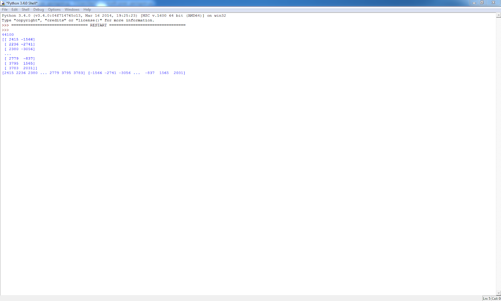
print(rate)
print(audData)
#wav bit type the amount of information recorded in each bit often 8, 16 or 32 bit
audData.dtype
#wav length
audData.shape[0] / rate
#wav number of channels mono/stereo
audData.shape[1]
#if stereo grab both channels
channel1=audData[:,0] #left
channel2=audData[:,1] #right
import numpy as np
#Energy of music np.sum(channel1.astype(float)**2)
#this can be infinite and depends on the length of the music of the loudness often talk about power
#power - energy per unit of time
1.0/(2*(channel1.size)+1)*np.sum(channel1.astype(float)**2)/rate
#save wav file
scipy.io.wavfile.write(temp_folder+"file2.wav", rate, audData)#save a file at half and double speed
scipy.io.wavfile.write(temp_folder+"file2.wav", rate/2, audData)
scipy.io.wavfile.write(temp_folder+"file2.wav", rate*2, audData)
#save a single channel
scipy.io.wavfile.write(temp_folder+"file2.wav", rate, channel1)
#averaging the channels damages the music
mono=np.sum(audData.astype(float), axis=1)/2
scipy.io.wavfile.write(temp_folder+"file2.wav", rate, mono)
import matplotlib.pyplot as plt
time = np.arange(0, float(audData.shape[0]), 1) / rate #plot amplitude (or loudness) over time
plt.figure(1)
plt.subplot(211)
plt.plot(time, channel1, linewidth=0.02, alpha=0.7, color='#ff7f00')
plt.xlabel('Time (s)')
plt.ylabel('Amplitude')
plt.subplot(212)
plt.plot(time, channel2, linewidth=0.02, alpha=0.7, color='#ff7f00')
plt.xlabel('Time (s)')
plt.ylabel('Amplitude')
plt.savefig(temp_folder+'ampiltude.png', bbox_inches='tight')
#Frequency (pitch) over time
#a fourier transform breaks the sound wave into series of waves that make up the main sound wave
#each of these waves will have its own amplitude (volume) and frequency. The frequency is the length over which the wave repeats itself. this is known as the pitch of the sound
from numpy import fft as fft
fourier=fft.fft(channel1)
plt.figure(1, figsize=(8,6))
plt.plot(fourier, color='#ff7f00')
plt.xlabel('k')
plt.ylabel('Amplitude')
plt.savefig(temp_folder+'fft.png', bbox_inches='tight')
n = len(channel1)
fourier = fourier[0:(n/2)]
# scale by the number of points so that the magnitude does not depend on the length
fourier = fourier / float(n)
#calculate the frequency at each point in Hz
freqArray = np.arange(0, (n/2), 1.0) * (rate*1.0/n);
plt.figure(1, figsize=(8,6))
plt.plot(freqArray/1000, 10*np.log10(fourier), color='#ff7f00', linewidth=0.02)
plt.xlabel('Frequency (kHz)')
plt.ylabel('Power (dB)')
plt.savefig(temp_folder+'frequencies.png', bbox_inches='tight')
#the function calculates many fft's over NFFT sized blocks of data
#increasing NFFT gives you a more detail across the spectrum range but decreases the samples per second
#the sampling rate used determines the frequency range seen always 0 to rate/2
plt.figure(2, figsize=(8,6))
plt.subplot(211)
Pxx, freqs, bins, im = plt.specgram(channel1, Fs=rate, NFFT=1024, cmap=plt.get_cmap('autumn_r'))
cbar=plt.colorbar(im)
plt.xlabel('Time (s)')
plt.ylabel('Frequency (Hz)')
cbar.set_label('Intensity dB')
plt.subplot(212)
Pxx, freqs, bins, im = plt.specgram(channel2, Fs=rate, NFFT=1024, cmap=plt.get_cmap('autumn_r'))
cbar=plt.colorbar(im)
plt.xlabel('Time (s)')
plt.ylabel('Frequency (Hz)')
cbar.set_label('Intensity (dB)')
#plt.show()
plt.savefig(temp_folder+'spectogram.png', bbox_inches='tight')
#Smaller Window Size value increases time resolution
#Specify a Frequency Range to be calculated for using the Goertzel function
#Specify which axis to put frequency
Pxx, freqs, timebins, im = plt.specgram(channel2, Fs=rate, NFFT=1024, noverlap=0, cmap=plt.get_cmap('autumn_r'))
channel1.shape
Pxx.shape
freqs.shape
timebins.shape
np.min(freqs)
np.max(freqs)
np.min(timebins)
np.max(timebins)
np.where(freqs==10034.47265625)
MHZ10=Pxx[233,:]
plt.figure(figsize=(8,6))
plt.plot(timebins, MHZ10, color='#ff7f00')
plt.savefig(temp_folder+'MHZ10.png', bbox_inches='tight')
But,there is a error on Orange lines as source.Execute conclusion as screenshot-1

Thus,I produced to most good condition for Program
TEST_2
#required libraries
import urllib.request
import scipy.io.wavfile
from pydub import AudioSegment
import pydub
#a temp folder for downloads
temp_folder="/Users/Geo/Desktop/"
#spotify mp3 sample file
web_file="http://p.scdn.co/mp3-preview/35b4ce45af06203992a86fa729d17b1c1f93cac5"
#download file
urllib.request.urlretrieve(web_file,temp_folder+"file.mp3")
#read mp3 file
AudioSegment.converter = "/ffmpeg/bin/ffmpeg"
mp3 = pydub.AudioSegment.from_mp3(temp_folder+"file.mp3")
#convert to wav
mp3.export(temp_folder+"file.wav", format="wav")
#read wav file
rate,audData=scipy.io.wavfile.read(temp_folder+"file.wav")
#the sample rate is the number of bits of information recorded per second
print(rate)
print(audData)
#wav bit type the amount of information recorded in each bit often 8, 16 or 32 bit
audData.dtype
#wav length
audData.shape[0] / rate
#wav number of channels mono/stereo
audData.shape[1]
#if stereo grab both channels
channel1=audData[:,0] #left
channel2=audData[:,1] #right
import numpy as np
#Energy of music
np.sum(channel1.astype(float)**2)
#this can be infinite and depends on the length of the music of the loudness often talk about power
#power - energy per unit of time
1.0/(2*(channel1.size)+1)*np.sum(channel1.astype(float)**2)/rate
#save a single channel
scipy.io.wavfile.write(temp_folder+"file2.wav", rate, channel1)
#averaging the channels damages the music
mono=np.sum(audData.astype(float), axis=1)/2
scipy.io.wavfile.write(temp_folder+"file2.wav", rate, mono)
import matplotlib.pyplot as plt
time = np.arange(0, float(audData.shape[0]), 1) / rate
#plot amplitude (or loudness) over time
plt.figure(1)
plt.subplot(211)
plt.plot(time, channel1, linewidth=0.02, alpha=0.7, color='#ff7f00')
plt.xlabel('Time (s)')
plt.ylabel('Amplitude')
plt.subplot(212)
plt.plot(time, channel2, linewidth=0.02, alpha=0.7, color='#ff7f00')
plt.xlabel('Time (s)')
plt.ylabel('Amplitude')
plt.savefig(temp_folder+'ampiltude.png', bbox_inches='tight')
#Frequency (pitch) over time
#a fourier transform breaks the sound wave into series of waves that make up the main sound wave
#each of these waves will have its own amplitude (volume) and frequency. The frequency is the length over which the wave repeats itself. this is known as the pitch of the sound
from numpy import fft as fft
fourier=fft.fft(channel1)
plt.figure(1, figsize=(8,6))
plt.plot(fourier, color='#ff7f00')
plt.xlabel('k')
plt.ylabel('Amplitude')
plt.savefig(temp_folder+'fft.png', bbox_inches='tight')
#plot spectogram
#the function calculates many fft's over NFFT sized blocks of data
#increasing NFFT gives you a more detail across the spectrum range but decreases the samples per second
#the sampling rate used determines the frequency range seen always 0 to rate/2
plt.figure(2, figsize=(8,6))
plt.subplot(211)
Pxx, freqs, bins, im = plt.specgram(channel1, Fs=rate, NFFT=1024, cmap=plt.get_cmap('autumn_r'))
cbar=plt.colorbar(im)
plt.xlabel('Time (s)')
plt.ylabel('Frequency (Hz)')
cbar.set_label('Intensity dB')
plt.subplot(212)
Pxx, freqs, bins, im = plt.specgram(channel2, Fs=rate, NFFT=1024, cmap=plt.get_cmap('autumn_r'))
cbar=plt.colorbar(im)
plt.xlabel('Time (s)')
plt.ylabel('Frequency (Hz)')
cbar.set_label('Intensity (dB)')
plt.show()
plt.savefig(temp_folder+'spectogram.png', bbox_inches='tight')
#Larger Window Size value increases frequency resolution
#Smaller Window Size value increases time resolution
#Specify a Frequency Range to be calculated for using the Goertzel function
#Specify which axis to put frequency
Pxx, freqs, timebins, im = plt.specgram(channel2, Fs=rate, NFFT=1024, noverlap=0, cmap=plt.get_cmap('autumn_r'))
Pxx.shape
freqs.shape
timebins.shape
np.min(freqs)
np.max(freqs)
np.min(timebins)
np.max(timebins)
np.where(freqs==10034.47265625)
MHZ10=Pxx[233,:]
plt.figure(figsize=(8,6))
plt.plot(timebins, MHZ10, color='#ff7f00')
plt.savefig(temp_folder+'MHZ10.png', bbox_inches='tight')
about applicable solutions for TEST_1 that your answers thus will be quite important...
Note:ffmpeg is requiring for pydub module.For installing procedure;
https://www.youtube.com/watch?v=xcdTIDHm4KM
Also,temp_folder as route is important
-----------------------------------------------------------------------------------------------------------------
Again Hello!(I work as dense and thus there are important developments for program).I present new condition;
Note:My procedure this time with print(x) approaches.Thus,background colours that have expressed as different than before tests.And,finally,error line for program that redline...So,
plt.plot(freqArray/1000, 10*np.log10(fourier),color='#ff7f00', linewidth=0.02)
What is solution for Line?
Special Thanks for Answers....
#required libraries
import urllib.request
import scipy.io.wavfile
from pydub import AudioSegment
import pydub
#a temp folder for downloads
temp_folder="/Users/Geo/Desktop/"
#spotify mp3 sample file
web_file="https://p.scdn.co/mp3-preview/0ba9d38f5d1ad30f0e31fc8ee80c1bebf0345a0c"
#download file
urllib.request.urlretrieve(web_file,temp_folder+"file.mp3")
#read mp3 file
AudioSegment.converter = "/ffmpeg/bin/ffmpeg"
mp3 = pydub.AudioSegment.from_mp3(temp_folder+"file.mp3")
#convert to wav
mp3.export(temp_folder+"file.wav", format="wav")
#read wav file
rate,audData=scipy.io.wavfile.read(temp_folder+"file.wav")
#the sample rate is the number of bits of information recorded per second
print(rate)
print(audData)
#wav bit type the amount of information recorded in each bit often 8, 16 or 32 bit
audData.dtype
#wav length
audData.shape[0] / rate
#wav number of channels mono/stereo
audData.shape[1]
#if stereo grab both channels
channel1=audData[:,0] #left
channel2=audData[:,1] #right
print(channel1,channel2)
import numpy as np
#Energy of music
np.sum(channel1.astype(float)**2)
#this can be infinite and depends on the length of the music of the loudness often talk about power
#power - energy per unit of time
1.0/(2*(channel1.size)+1)*np.sum(channel1.astype(float)**2)/rate
#save wav file
scipy.io.wavfile.write(temp_folder+"file2.wav", rate, audData)
#save a file at half and double speed
#scipy.io.wavfile.write(temp_folder+"file2.wav", rate/2, audData)#This line is producing to error
scipy.io.wavfile.write(temp_folder+"file2.wav", rate*2, audData)
#save a single channel
scipy.io.wavfile.write(temp_folder+"file2.wav", rate, channel1)
#averaging the channels damages the music
mono=np.sum(audData.astype(float), axis=1)/2
scipy.io.wavfile.write(temp_folder+"file2.wav", rate, mono)
import matplotlib.pyplot as plt
time = np.arange(0, float(audData.shape[0]), 1) / rate
#plot amplitude (or loudness) over time
plt.figure(1)
plt.subplot(211)
plt.plot(time, channel1, linewidth=0.02, alpha=0.7, color='#ff7f00')
plt.xlabel('Time (s)')
plt.ylabel('Amplitude')
plt.subplot(212)
plt.plot(time, channel2, linewidth=0.02, alpha=0.7, color='#ff7f00')
plt.xlabel('Time (s)')
plt.ylabel('Amplitude')
plt.savefig(temp_folder+'ampiltude.png', bbox_inches='tight')
#Frequency (pitch) over time
#a fourier transform breaks the sound wave into series of waves that make up the main sound wave
#each of these waves will have its own amplitude (volume) and frequency. The frequency is the length over which the wave repeats itself. this is known as the pitch of the sound
from numpy import fft as fft
fourier=fft.fft(channel1)
plt.figure(1, figsize=(8,6))
plt.plot(fourier, color='#ff7f00')
plt.xlabel('k')
plt.ylabel('Amplitude')
plt.savefig(temp_folder+'fft.png', bbox_inches='tight')
#the fourier is symetrical due to the real and imaginary soultion. only interested in first real solution
n = len(channel1)
print(n)
fourier = fourier[0:(n*2)]#Note:n*2 is before n/2(n/2 thus presents error!!!)
nup=np.ceil((n+1)/2.0)#after error,nup line have realised
# scale by the number of points so that the magnitude does not depend on the length
fourier = fourier / float(n)
print(fourier)
#calculate the frequency at each point in Hz
freqArray = np.arange(0, (nup), 1.0) * (rate*1.0/n);#nup parameter is thisline!!!
print(freqArray)
plt.figure(1, figsize=(8,6))
plt.plot(freqArray/1000, 10*np.log10(fourier),color='#ff7f00', linewidth=0.02)
plt.xlabel('Frequency (kHz)')
plt.ylabel('Power (dB)')
plt.savefig(temp_folder+'frequencies.png', bbox_inches='tight')
#plot spectogram
#the function calculates many fft's over NFFT sized blocks of data
#increasing NFFT gives you a more detail across the spectrum range but decreases the samples per second
#the sampling rate used determines the frequency range seen always 0 to rate/2
plt.figure(2, figsize=(8,6))
plt.subplot(211)
Pxx, freqs, bins, im = plt.specgram(channel1, Fs=rate, NFFT=1024, cmap=plt.get_cmap('autumn_r'))
cbar=plt.colorbar(im)
plt.xlabel('Time (s)')
plt.ylabel('Frequency (Hz)')
cbar.set_label('Intensity dB')
plt.subplot(212)
Pxx, freqs, bins, im = plt.specgram(channel2, Fs=rate, NFFT=1024, cmap=plt.get_cmap('autumn_r'))
cbar=plt.colorbar(im)
plt.xlabel('Time (s)')
plt.ylabel('Frequency (Hz)')
cbar.set_label('Intensity (dB)')
#plt.show()
plt.savefig(temp_folder+'spectogram.png', bbox_inches='tight')
#Larger Window Size value increases frequency resolution
#Smaller Window Size value increases time resolution
#Specify a Frequency Range to be calculated for using the Goertzel function
#Specify which axis to put frequency
Pxx, freqs, timebins, im = plt.specgram(channel2, Fs=rate, NFFT=1024, noverlap=0, cmap=plt.get_cmap('autumn_r'))
channel1.shape
Pxx.shape
freqs.shape
timebins.shape
np.min(freqs)
np.max(freqs)
np.min(timebins)
np.max(timebins)
np.where(freqs==10034.47265625)
MHZ10=Pxx[233,:]
plt.figure(figsize=(8,6))
plt.plot(timebins, MHZ10, color='#ff7f00')
plt.savefig(temp_folder+'MHZ10.png', bbox_inches='tight')
for execute conclusions

--------------------------------------------------------------------------------------------------------------------
about Program that all errors as possible as a conclusion of my dense working have solutioned...
By the way,rate/2------>solutioning as int(rate/2) .Full conclusion with my other corrections have carried-out;
#required libraries
import urllib.request
import scipy.io.wavfile
from pydub import AudioSegment
import pydub
#a temp folder for downloads
temp_folder="/Users/Geo/Desktop/"
#spotify mp3 sample file
web_file="https://p.scdn.co/mp3-preview/0ba9d38f5d1ad30f0e31fc8ee80c1bebf0345a0c"
#download file
urllib.request.urlretrieve(web_file,temp_folder+"file.mp3")
#read mp3 file
AudioSegment.converter = "/ffmpeg/bin/ffmpeg"
mp3 = pydub.AudioSegment.from_mp3(temp_folder+"file.mp3")
#convert to wav
mp3.export(temp_folder+"file.wav", format="wav")
#read wav file
rate,audData=scipy.io.wavfile.read(temp_folder+"file.wav")
#the sample rate is the number of bits of information recorded per second
print(rate)
print(audData)
#wav bit type the amount of information recorded in each bit often 8, 16 or 32 bit
audData.dtype
#wav length
audData.shape[0] / rate
#wav number of channels mono/stereo
audData.shape[1]
#if stereo grab both channels
channel1=audData[:,0] #left
channel2=audData[:,1] #right
print(channel1,channel2)
import numpy as np
#Energy of music
np.sum(channel1.astype(float)**2)
#this can be infinite and depends on the length of the music of the loudness often talk about power
#power - energy per unit of time
1.0/(2*(channel1.size)+1)*np.sum(channel1.astype(float)**2)/rate
#save wav file
scipy.io.wavfile.write(temp_folder+"file2.wav", rate, audData)
#save a file at half and double speed
scipy.io.wavfile.write(temp_folder+"file2.wav", int(rate/2), audData)
scipy.io.wavfile.write(temp_folder+"file2.wav", rate*2, audData)
#save a single channel
scipy.io.wavfile.write(temp_folder+"file2.wav", rate, channel1)
#averaging the channels damages the music
mono=np.sum(audData.astype(float), axis=1)/2
scipy.io.wavfile.write(temp_folder+"file2.wav", rate, mono)
import matplotlib.pyplot as plt
time = np.arange(0, float(audData.shape[0]), 1) / rate
#plot amplitude (or loudness) over time
plt.figure(1)
plt.subplot(211)
plt.plot(time, channel1, linewidth=0.02, alpha=0.7, color='#ff7f00')
plt.xlabel('Time (s)')
plt.ylabel('Amplitude')
plt.subplot(212)
plt.plot(time, channel2, linewidth=0.02, alpha=0.7, color='#ff7f00')
plt.xlabel('Time (s)')
plt.ylabel('Amplitude')
plt.savefig(temp_folder+'ampiltude.png', bbox_inches='tight')
#Frequency (pitch) over time
#a fourier transform breaks the sound wave into series of waves that make up the main sound wave
#each of these waves will have its own amplitude (volume) and frequency. The frequency is the length over which the wave repeats itself. this is known as the pitch of the sound
from numpy import fft as fft
fourier=fft.fft(channel1)
plt.figure(1, figsize=(8,6))
plt.plot(fourier, color='#ff7f00')
plt.xlabel('k')
plt.ylabel('Amplitude')
plt.savefig(temp_folder+'fft.png', bbox_inches='tight')
#the fourier is symetrical due to the real and imaginary soultion. only interested in first real solution
n = len(channel1)
print(n)
fourier = fourier[0:(n*2)]#Note:n*2 is before n/2(n/2 thus presents error!!!)
nup=np.ceil((n+1)/2.0)#after error,nup line have realised
# scale by the number of points so that the magnitude does not depend on the length
fourier = fourier / float(n)
print(fourier)
#calculate the frequency at each point in Hz
freqArray = np.arange(0, (nup), 1.0) * (rate*1.0/n);#nup parameter is thisline!!!
print(freqArray)
yu=freqArray/1000
print(yu)
say0=len(yu)
print(say0)
bu=10*np.log10(fourier)
print(bu)
Z=(bu.real,bu.imag)
print(Z)
A=bu.real
B=bu.imag
print(A)
print(B)
say1=len(A)
say2=len(B)
print(say1)
print(say2)
yu=np.concatenate([yu,np.zeros(661499)])
print(yu)
plt.plot(yu,A,color='#ff7f00', linewidth=0.02)
plt.xlabel('Frequency (kHz)')
plt.ylabel('Power (dB)')
plt.savefig(temp_folder+'frequencies.png', bbox_inches='tight')
#plot spectogram
#the function calculates many fft's over NFFT sized blocks of data
#increasing NFFT gives you a more detail across the spectrum range but decreases the samples per second
#the sampling rate used determines the frequency range seen always 0 to rate/2
plt.figure(2, figsize=(8,6))
plt.subplot(211)
Pxx, freqs, bins, im = plt.specgram(channel1, Fs=rate, NFFT=1024, cmap=plt.get_cmap('autumn_r'))
cbar=plt.colorbar(im)
plt.xlabel('Time (s)')
plt.ylabel('Frequency (Hz)')
cbar.set_label('Intensity dB')
plt.subplot(212)
Pxx, freqs, bins, im = plt.specgram(channel2, Fs=rate, NFFT=1024, cmap=plt.get_cmap('autumn_r'))
cbar=plt.colorbar(im)
plt.xlabel('Time (s)')
plt.ylabel('Frequency (Hz)')
cbar.set_label('Intensity (dB)')
#plt.show()
plt.savefig(temp_folder+'spectogram.png', bbox_inches='tight')
#Larger Window Size value increases frequency resolution
#Smaller Window Size value increases time resolution
#Specify a Frequency Range to be calculated for using the Goertzel function
#Specify which axis to put frequency
Pxx, freqs, timebins, im = plt.specgram(channel2, Fs=rate, NFFT=1024, noverlap=0, cmap=plt.get_cmap('autumn_r'))
channel1.shape
Pxx.shape
freqs.shape
timebins.shape
np.min(freqs)
np.max(freqs)
np.min(timebins)
np.max(timebins)
np.where(freqs==10034.47265625)
MHZ10=Pxx[233,:]
plt.figure(figsize=(8,6))
plt.plot(timebins, MHZ10, color='#ff7f00')
plt.savefig(temp_folder+'MHZ10.png', bbox_inches='tight')


In the other hand,I am not hearing any sound for file2 file.I wonder thus,this condition normal
------------------------------------------------------------------------------------------------------------------------
Conclusion as all with Latest program is positive.But,about Power spectogram you know there is problem.I realised thus a conclusion;
#required libraries
import urllib.request
import scipy.io.wavfile
from pydub import AudioSegment
import pydub
#a temp folder for downloads
temp_folder="/Users/Geo/Desktop/"
#spotify mp3 sample file
web_file="https://p.scdn.co/mp3-preview/0ba9d38f5d1ad30f0e31fc8ee80c1bebf0345a0c"
#download file
urllib.request.urlretrieve(web_file,temp_folder+"file.mp3")
#read mp3 file
AudioSegment.converter = "/ffmpeg/bin/ffmpeg"
mp3 = pydub.AudioSegment.from_mp3(temp_folder+"file.mp3")
#convert to wav
mp3.export(temp_folder+"file.wav", format="wav")
#read wav file
rate,audData=scipy.io.wavfile.read(temp_folder+"file.wav")
#the sample rate is the number of bits of information recorded per second
print(rate)
print(audData)
#wav bit type the amount of information recorded in each bit often 8, 16 or 32 bit
audData.dtype
#wav length
audData.shape[0] / rate
#wav number of channels mono/stereo
audData.shape[1]
#if stereo grab both channels
channel1=audData[:,0] #left
channel2=audData[:,1] #right
print(channel1,channel2)
import numpy as np
#Energy of music
np.sum(channel1.astype(float)**2)
#this can be infinite and depends on the length of the music of the loudness often talk about power
#power - energy per unit of time
1.0/(2*(channel1.size)+1)*np.sum(channel1.astype(float)**2)/rate
#save wav file
scipy.io.wavfile.write(temp_folder+"file2.wav", rate, audData)
#save a file at half and double speed
scipy.io.wavfile.write(temp_folder+"file2.wav", int(rate/2), audData)
scipy.io.wavfile.write(temp_folder+"file2.wav", rate*2, audData)
#save a single channel
scipy.io.wavfile.write(temp_folder+"file2.wav", rate, channel1)
#averaging the channels damages the music
mono=np.sum(audData.astype(float), axis=1)/2
scipy.io.wavfile.write(temp_folder+"file2.wav", rate, mono)
import matplotlib.pyplot as plt
time = np.arange(0, float(audData.shape[0]), 1) / rate
#plot amplitude (or loudness) over time
plt.figure(1)
plt.subplot(211)
plt.plot(time, channel1, linewidth=0.02, alpha=0.7, color='#ff7f00')
plt.xlabel('Time (s)')
plt.ylabel('Amplitude')
plt.subplot(212)
plt.plot(time, channel2, linewidth=0.02, alpha=0.7, color='#ff7f00')
plt.xlabel('Time (s)')
plt.ylabel('Amplitude')
plt.savefig(temp_folder+'ampiltude.png', bbox_inches='tight')
#Frequency (pitch) over time
#a fourier transform breaks the sound wave into series of waves that make up the main sound wave
#each of these waves will have its own amplitude (volume) and frequency. The frequency is the length over which the wave repeats itself. this is known as the pitch of the sound
from numpy import fft as fft
fourier=fft.fft(channel1)
plt.figure(1, figsize=(8,6))
plt.plot(fourier, color='#ff7f00')
plt.xlabel('k')
plt.ylabel('Amplitude')
plt.savefig(temp_folder+'fft.png', bbox_inches='tight')
#the fourier is symetrical due to the real and imaginary soultion. only interested in first real solution
n = len(channel1)
print(n)
fourier = fourier[0:(n*2)]#Note:n*2 is before n/2(n/2 thus presents error!!!)
nup=np.ceil((n+1)/2.0)#after error,nup line have realised
# scale by the number of points so that the magnitude does not depend on the length
fourier = fourier / float(n)
print(fourier)
#calculate the frequency at each point in Hz
freqArray = np.arange(0, (nup), 1.0) * (rate*1.0/n);#nup parameter is thisline!!!
print(freqArray)
yu=freqArray/1000
print(yu)
say0=len(yu)
print(say0)
bu=10*np.log10(fourier)
print(bu)
Z=(bu.real,bu.imag)
print(Z)
A=bu.real
B=bu.imag
print(A)
print(B)
say1=len(A)
say2=len(B)
print(say1)
print(say2)
yu=np.concatenate([yu,np.zeros(661499)])
print(yu)
plt.plot(yu,A,color='#ff7f00', linewidth=0.02)
plt.xlabel('Frequency (kHz)')
plt.ylabel('Power (dB)')
plt.savefig(temp_folder+'frequencies.png', bbox_inches='tight')
#plot spectogram
#the function calculates many fft's over NFFT sized blocks of data
#increasing NFFT gives you a more detail across the spectrum range but decreases the samples per second
#the sampling rate used determines the frequency range seen always 0 to rate/2
plt.figure(2, figsize=(8,6))
plt.subplot(211)
Pxx, freqs, bins, im = plt.specgram(channel1, Fs=rate, NFFT=1024, cmap=plt.get_cmap('autumn_r'))
cbar=plt.colorbar(im)
plt.xlabel('Time (s)')
plt.ylabel('Frequency (Hz)')
cbar.set_label('Intensity dB')
plt.subplot(212)
Pxx, freqs, bins, im = plt.specgram(channel2, Fs=rate, NFFT=1024, cmap=plt.get_cmap('autumn_r'))
cbar=plt.colorbar(im)
plt.xlabel('Time (s)')
plt.ylabel('Frequency (Hz)')
cbar.set_label('Intensity (dB)')
#plt.show()
plt.savefig(temp_folder+'spectogram.png', bbox_inches='tight')
#Larger Window Size value increases frequency resolution
#Smaller Window Size value increases time resolution
#Specify a Frequency Range to be calculated for using the Goertzel function
#Specify which axis to put frequency
Pxx, freqs, timebins, im = plt.specgram(channel2, Fs=rate, NFFT=1024, noverlap=0, cmap=plt.get_cmap('autumn_r'))
channel1.shape
Pxx.shape
freqs.shape
timebins.shape
np.min(freqs)
np.max(freqs)
np.min(timebins)
np.max(timebins)
np.where(freqs==10034.47265625)
MHZ10=Pxx[233,:]
plt.figure(figsize=(8,6))
plt.plot(timebins, MHZ10, color='#ff7f00')
plt.savefig(temp_folder+'MHZ10.png', bbox_inches='tight')
plt.show()
pwr=channel1/(yu**2)
plt.plot(yu,pwr,'r-')
plt.ylabel('power')
plt.xlabel('frequency')
plt.axis([0,23,0,100000000])
plt.show()
And,some outputs for power spectogram;


(as orginal)
Note:I evaluated function as a test. P=A/(f^2) .Also,fc have not evaluated for function.
You know also other P for Channel2
-----------------------------------------------------------------------------------------------------------------
This time,I wonder for EM Sound Patern...for aiming to this,I think Mummers Dance of Loreena McKennitt that last phase of record quite suitable...
-----------------------------------------------------------------------------------------------------------------
I realised new mp3 file as input;
#spotify mp3 sample file
web_file="https://p.scdn.co/mp3-preview/4ab65f9b193ccc37f2059344322462ae5e9dac90"
I still wait for conclusion:)(Laptop Cooler quite angry to me).I would like to present my waiting screen as a screenshot

I wait for your solutions...Thanks...There are some suggestions.Thus,I compiled for 3.6.3 64 Bit version.So,again same conditions.
-------------------------------------------------------------------------------------------------------------------
I established to caused point to CPU performance on step by step methodology.So,chapter is FT.
Thus,I discharged to numpy methodology on which using to scipy methodology;
#required libraries
import urllib.request
import scipy.io.wavfile
from pydub import AudioSegment
import pydub
#a temp folder for downloads
temp_folder="/Users/Geo/Desktop/"
#spotify mp3 sample file
web_file="https://p.scdn.co/mp3-preview/4ab65f9b193ccc37f2059344322462ae5e9dac90"
#download file
urllib.request.urlretrieve(web_file,temp_folder+"file.mp3")
#read mp3 file
AudioSegment.converter = "/ffmpeg/bin/ffmpeg"
mp3 = pydub.AudioSegment.from_mp3(temp_folder+"file.mp3")
#convert to wav
mp3.export(temp_folder+"file.wav", format="wav")
#read wav file
rate,audData=scipy.io.wavfile.read(temp_folder+"file.wav")
#the sample rate is the number of bits of information recorded per second
print(rate)
print(audData)
#wav bit type the amount of information recorded in each bit often 8, 16 or 32 bit
audData.dtype
#wav length
audData.shape[0] / rate
#wav number of channels mono/stereo
audData.shape[1]
#if stereo grab both channels
channel1=audData[:,0] #left
channel2=audData[:,1] #right
print(channel1,channel2)
import numpy as np
#Energy of music
np.sum(channel1.astype(float)**2)
#this can be infinite and depends on the length of the music of the loudness often talk about power
#power - energy per unit of time
1.0/(2*(channel1.size)+1)*np.sum(channel1.astype(float)**2)/rate
#save wav file
scipy.io.wavfile.write(temp_folder+"file2.wav", rate, audData)
#save a file at half and double speed
scipy.io.wavfile.write(temp_folder+"file2.wav", int(rate/2), audData)
scipy.io.wavfile.write(temp_folder+"file2.wav", rate*2, audData)
#save a single channel
scipy.io.wavfile.write(temp_folder+"file2.wav", rate, channel1)
#averaging the channels damages the music
mono=np.sum(audData.astype(float), axis=1)/2
scipy.io.wavfile.write(temp_folder+"file2.wav", rate, mono)
import matplotlib.pyplot as plt
time = np.arange(0, float(audData.shape[0]), 1) / rate
#plot amplitude (or loudness) over time
plt.figure(1)
plt.subplot(211)
plt.plot(time, channel1, linewidth=0.02, alpha=0.7, color='#ff7f00')
plt.xlabel('Time (s)')
plt.ylabel('Amplitude')
plt.subplot(212)
plt.plot(time, channel2, linewidth=0.02, alpha=0.7, color='#ff7f00')
plt.xlabel('Time (s)')
plt.ylabel('Amplitude')
plt.savefig(temp_folder+'ampiltude.png', bbox_inches='tight')
#Frequency (pitch) over time
#a fourier transform breaks the sound wave into series of waves that make up the main sound wave
#each of these waves will have its own amplitude (volume) and frequency. The frequency is the length over which the wave repeats itself. this is known as the pitch of the sound
from scipy.fftpack import fft, ifft
fourier=np.allclose(fft(ifft(channel1)), channel1,e-10) # within numerical accuracy.
plt.figure(1, figsize=(8,6))
plt.plot(fourier, color='#ff7f00')
plt.xlabel('k')
plt.ylabel('Amplitude')
plt.savefig(temp_folder+'fft.png', bbox_inches='tight')
I tuned with numerical accuracy and alternatively to condition without numerical accuracy...But, similar problem;
Cooler again very angry...
------------------------------------------------------------------------------------------------------------------------
Thus,I think a solution as mathematical...I think for solution to problem that chapter "a optimisation via minimisation function for fft".I will work for scipy.optimize...
------------------------------------------------------------------------------------------------------------------------
I oriented to sklearn preprocessing as a conclusion of my Scipy.optimize studies that normalize in preprocessing library quite interesting.Thus,
plt.savefig(temp_folder+'ampiltude.png', bbox_inches='tight')
after line
from sklearn.preprocessing import normalize
norm1 = parameter / np.linalg.norm(parameter)
norm2 = normalize(parameter[:,np.newaxis], axis=0).ravel()
print(np.all(norm1 == norm2))
print(norm1)
print(norm2)
some parameter variations have applied.As a conclusion;

you see again cooler is despondent...Thus,my first think about preprocessing that using to other functions...So,well understanding as all to functions of preprocessing.
Principle aim for this application as add must be a synthesis of Matplotlib with FFMPEG.Thus,example
https://www.youtube.com/watch?v=Db3DWXqwey4
--------------------------------------------------------------------------------------------------------------------------
I especially expressed before starting
to this studying about requirement of applying
to a methodology for kriging points.Thus,a example have presented.Signal
processing application shortly that about a depth approximation via power
spectrum.(By the way,I concluded that my
computer have not to capabilities of a solution for Mummers Dance.Also,I am especially
expressing that I often encountered with
error types as memory errors during some calculations as add )
I am returning to first chapter
that I will clearly express to my aim…(I am waiting for your solutions at this
direction)
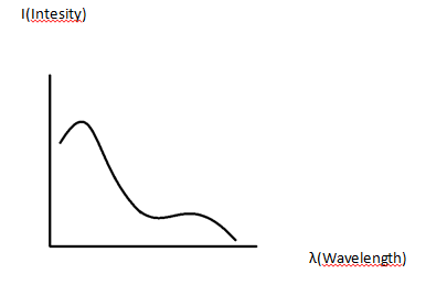
You know that
I=P/(4πr2)
Where;
I:Intensity
P:Power
r:distance as radius
Also,you know
P=B2/(2µ0) (I)
&
P=(µ0H2)/2 (II)
Where;
B:Magnetic Flux Density
H:Magnetic Field Density
Other steps;
B=E/c
c:Light Velocity,and E(Electric Field) is establishing
H=E/Z that Z(Impedance)
is establishing
that ε is establishing
J=σE
Where,σ=1/ρ and

In this conclusions,we know that Depth
Approximation from Power Spectrum at Geophysics.So,shortly;
Finally,decisioning with this conpcet of kriging points
(Note:I think that on this concept of signal process program will be useful)

Yorumlar
Yorum Gönder