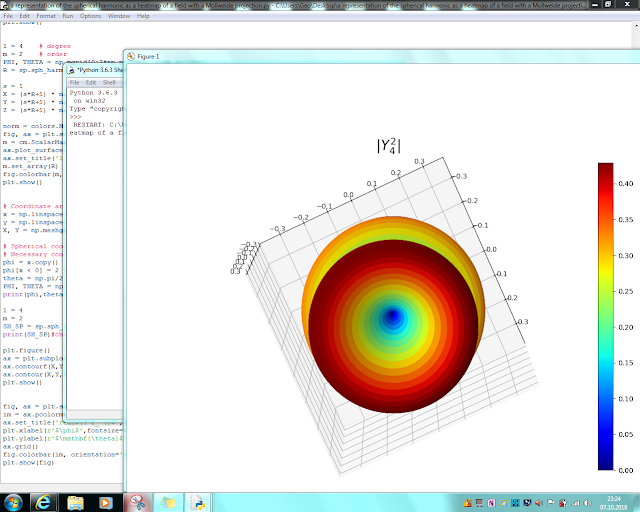
a representation of the spherical harmonic as a heatmap of a field with a Mollweide projection

Modelling Studies for Geophysicists quite important.Thus,A Globe Modelling Example which presenting on python programming language.Chapter as Summary;

expressing as a representation of the spherical harmonic as a heatmap of a field with a Mollweide projection

from __future__ import division
import scipy as sci
import scipy.special as sp
import numpy as np
import matplotlib
import matplotlib.pyplot as plt
from mpl_toolkits.mplot3d import Axes3D
from matplotlib import cm, colors

#Example to calculate Y_4^2
l = 4
m = 2
theta, phi = 0.6, 0.75    # Some arbitrary values of angles in radians
Y42 = sp.sph_harm(m, l, phi, theta)
z = np.cos(theta)
P42 = sp.lpmv(m,l,z)

f = sci.math.factorial
K_norm = np.sqrt((2*l+1)/(4 * np.pi) * f(l-m)/f(l+m))
K_norm * P42* np.exp(m*phi*1j) == Y42
def dotprod(f,g):
    #Scipy does not directly integrates complex functions.
    #You have to break them down into two integrals of the real and imaginary part
    integrand_r = lambda theta, phi: np.real(f(theta, phi) * np.conj(g(theta, phi)) * np.sin(theta))
    integrand_i = lambda theta, phi: np.imag(f(theta, phi) * np.conj(g(theta, phi)) * np.sin(theta))
    rr = sci.integrate.dblquad(integrand_r, 0, 2 * np.pi,lambda theta: 0, lambda theta: np.pi)[0]
    ri = sci.integrate.dblquad(integrand_i, 0, 2 * np.pi,lambda theta: 0, lambda theta: np.pi)[0]
    if np.allclose(rr,0):
        rr = 0
    if np.allclose(ri,0):
        ri=0
    return rr + ri*1j
#We check the orthogonality of the spherical harmonics:
# Si (l,m) =! (l',m') the inner product must be zero
Y = lambda l, m, theta, phi: sp.sph_harm(m, l, phi, theta)
f = lambda theta, phi: Y(4,3,theta, phi)
g = lambda theta, phi: Y(4,2,theta, phi)
#And, if (l,m) = (l',m') the inner product is one.
f = lambda theta, phi: Y(4,3,theta, phi)
g = lambda theta, phi: Y(4,3,theta, phi)

l = 4    #degree
m = 2    # order
PHI, THETA = np.mgrid[0:2*np.pi:200j, 0:np.pi:100j] #arrays of angular variables
R = np.abs(sp.sph_harm(m, l, PHI, THETA)) #Array with the absolute values of Ylm
#Now we convert to cartesian coordinates
# for the 3D representation
X = R * np.sin(THETA) * np.cos(PHI)
Y = R * np.sin(THETA) * np.sin(PHI)
Z = R * np.cos(THETA)
N = R/R.max()    # Normalize R for the plot colors to cover the entire range of colormap.
fig, ax = plt.subplots(subplot_kw=dict(projection='3d'), figsize=(12,10))
im = ax.plot_surface(X, Y, Z, rstride=1, cstride=1, facecolors=cm.jet(N))
ax.set_title(r'$|Y^2_ 4|$', fontsize=20)
m = cm.ScalarMappable(cmap=cm.jet)
m.set_array(R)    # Assign the unnormalized data array to the mappable
                  #so that the scale corresponds to the values of R
fig.colorbar(m, shrink=0.8);
plt.show()

l = 4    # degree
m = 2    # order
PHI, THETA = np.mgrid[0:2*np.pi:200j, 0:np.pi:100j]
R = sp.sph_harm(m, l, PHI, THETA).real
X = R * np.sin(THETA) * np.cos(PHI)
Y = R * np.sin(THETA) * np.sin(PHI)
Z = R * np.cos(THETA)
#As R has negative values, we'll use an instance of Normalize
#see http://stackoverflow.com/questions/25023075/normalizing-colormap-used-by-facecolors-in-matplotlib
norm = colors.Normalize()
fig, ax = plt.subplots(subplot_kw=dict(projection='3d'), figsize=(14,10))
m = cm.ScalarMappable(cmap=cm.jet)
ax.plot_surface(X, Y, Z, rstride=1, cstride=1, facecolors=cm.jet(norm(R)))
ax.set_title('real$(Y^2_ 4)$', fontsize=20)
m.set_array(R)
fig.colorbar(m, shrink=0.8);
plt.show()

l = 4    # degree
m = 2    # order
PHI, THETA = np.mgrid[0:2*np.pi:300j, 0:np.pi:150j]
R = sp.sph_harm(m, l, PHI, THETA).real
s = 1
X = (s*R+1) * np.sin(THETA) * np.cos(PHI)
Y = (s*R+1) * np.sin(THETA) * np.sin(PHI)
Z = (s*R+1) * np.cos(THETA)
norm = colors.Normalize()
fig, ax = plt.subplots(subplot_kw=dict(projection='3d'), figsize=(14,10))
m = cm.ScalarMappable(cmap=cm.jet)
ax.plot_surface(X, Y, Z, rstride=1, cstride=1, facecolors=cm.jet(norm(R)))
ax.set_title('1 + real$(Y^2_ 4)$', fontsize=20)
m.set_array(R)
fig.colorbar(m, shrink=0.8);
plt.show()

# Coordinate arrays for the graphical representation
x = np.linspace(-np.pi, np.pi, 100)
y = np.linspace(-np.pi/2, np.pi/2, 50)
X, Y = np.meshgrid(x, y)
# Spherical coordinate arrays derived from x, y
# Necessary conversions to get Mollweide right
phi = x.copy()    # physical copy
phi[x < 0] = 2 * np.pi + x[x<0]
theta = np.pi/2 - y
PHI, THETA = np.meshgrid(phi, theta)
print(phi,theta)#checking to Phi and Theta values
l = 4
m = 2
SH_SP = sp.sph_harm(m, l, PHI, THETA).real    # Plot just the real part
print(SH_SP)#checking to Just Real Part
plt.figure()
ax = plt.subplot(111, projection = 'mollweide')
ax.contourf(X,Y,SH_SP,100)
ax.contour(X,Y,SH_SP,10,colors='k')
plt.show()

fig, ax = plt.subplots(subplot_kw=dict(projection='mollweide'), figsize=(10,8))
im = ax.pcolormesh(X, Y , SH_SP,cmap=cm.jet)#For example,using as cmap="Spectral",cmap="seismic",cmap="coolwarm" as other alternatives
ax.set_title('real$(Y^2_ 4)$', fontsize=20,fontweight='bold')
plt.xlabel(r'$\phi$',fontsize=20)#Italic font method
plt.ylabel(r'$\mathbf{\theta}$',fontsize=20)#Bold font method without fontweight parameters
ax.grid()
fig.colorbar(im, orientation='horizontal');
plt.show(fig)

Unfortunately,I have not been realised to any solutions for 3D analysis perfomance.Absolute value and some snapshots about real part are presenting;