Obspy-about Developments
Orfeus as European Infrastructure for Seismic Waveform in European Observating System on AlpArray Initiative is knowing on Seismologic Infrastructure Studies into European Hinterland.
New vision that shortly,expressing as "Synergy"
With this aim,widening of organisational structure is basepoint.For this,emphasizing to powerfulness of a "mass approach" on observing of European Hinterland on opensource programming language
As a conclusion of efforts in this field,a "Data Network Structure System" on Obspy&Python Programming Capabilities have developed.
Shortly,reading on internet network of basedata &carrying-out by user of some data process steps.And next,presenting on some types of some conclusions...
So,summarying as "Platform Structure"
On earthquake researches,providing to international a "synergy" on ground researches besides earthquake via user networks at hinterland countries for establishing as powerful of infrastructure can express.
I realised to some evaluations based on Obspy;
from obspy.core.util.base import get_example_file
 A pre-information about Frequency Analysis Capabilities on Amplitude-Time
 A example for file exporting on file formats(Where,for example 92/92 segment data for your analysis is showing on your defining)


Other presentation examples of 47/47 and 93/93 segments(A and B) for your data analysis studies

Amplitude-Period example of 93/93 Segment for your Data Analysis Studies

Amplitude-Period example as non-exceedance as cumulative of 93/93 Segment for your Data Analysis Studies

Amplitude Spectogram on Period-Time
from obspy.signal.tf_misfit import plot_tf_gofs
# amplitude and phase error
# reference signal


import numpy as np
# Filtering the Stream object

import obspy
Example:
Interval=80
Interval=30
Magnitude Min=4.0
Conclusions of a working on events;
import numpy as np
# Read the seismogram
scalogram = cwt(tr.data, dt, 8, f_min, f_max)
fig = plt.figure()

tr = obspy.read("https://examples.obspy.org/a02i.2008.240.mseed")[0]
fig = plt.figure()

import matplotlib.pyplot as plt
cmap = obspy_sequential
# make output human readable, adjust backazimuth to values between 0 and 360


*Curves as Time(mimutes)-Distance(degree) of P-PP-S
from obspy.taup import plot_travel_times
import matplotlib.pyplot as plt
fig, ax = plt.subplots()
ax = plot_travel_times(source_depth=10, ax=ax, fig=fig,
phase_list=['P', 'PP', 'S'], npoints=200)

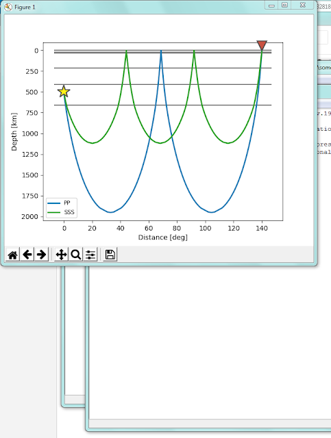
*Depth(km)-Distance(degree) Modelling as Sectional
from obspy.taup import TauPyModel
model = TauPyModel(model='iasp91')
arrivals = model.get_ray_paths(500, 140, phase_list=['PP', 'SSS'])
arrivals.plot_rays(plot_type='cartesian', phase_list=['PP', 'SSS'],
plot_all=False, legend=True)
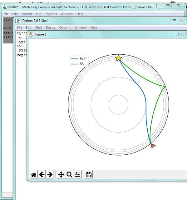
*Pfdiff&SS Modelling Example on Earth Section
from obspy.taup import TauPyModel
model = TauPyModel(model='iasp91')
arrivals = model.get_ray_paths(500, 140, phase_list=['Pdiff', 'SS'])
arrivals.plot_rays(plot_type='spherical', phase_list=['Pdiff', 'SS'],
legend=True)
*Phase Distances
import numpy as np
import matplotlib.pyplot as plt
from obspy.taup import TauPyModel
PHASES = [
# Phase, distance
('P', 26),
('PP', 60),
('PPP', 94),
('PPS', 155),
('p', 3),
('pPcP', 100),
('PKIKP', 170),
('PKJKP', 194),
('S', 65),
('SP', 85),
('SS', 134.5),
('SSS', 204),
('p', -10),
('pP', -37.5),
('s', -3),
('sP', -49),
('ScS', -44),
('SKS', -82),
('SKKS', -120),
]
model = TauPyModel(model='iasp91')
fig, ax = plt.subplots(subplot_kw=dict(polar=True))
# Plot all pre-determined phases
for phase, distance in PHASES:
arrivals = model.get_ray_paths(700, distance, phase_list=[phase])
ax = arrivals.plot_rays(plot_type='spherical',
legend=False, label_arrivals=True,
plot_all=True,
show=False, ax=ax)
# Annotate regions
ax.text(0, 0, 'Solid\ninner\ncore',
horizontalalignment='center', verticalalignment='center',
bbox=dict(facecolor='white', edgecolor='none', alpha=0.7))
ocr = (model.model.radius_of_planet -
(model.model.s_mod.v_mod.iocb_depth +
model.model.s_mod.v_mod.cmb_depth) / 2)
ax.text(np.deg2rad(180), ocr, 'Fluid outer core',
horizontalalignment='center',
bbox=dict(facecolor='white', edgecolor='none', alpha=0.7))
mr = model.model.radius_of_planet - model.model.s_mod.v_mod.cmb_depth / 2
ax.text(np.deg2rad(180), mr, 'Solid mantle',
horizontalalignment='center',
bbox=dict(facecolor='white', edgecolor='none', alpha=0.7))
plt.show()

*Raypath Modelling Example of P&PKP Phases
from obspy.taup.tau import plot_ray_paths
import matplotlib.pyplot as plt
fig, ax = plt.subplots(subplot_kw=dict(polar=True))
ax = plot_ray_paths(source_depth=100, ax=ax, fig=fig, phase_list=['P', 'PKP'],
npoints=25)

**about plotting as a conclusion of processes on producing to array coordinates
import numpy as np
import matplotlib.pyplot as plt
from obspy.imaging.cm import obspy_sequential
from obspy.signal.array_analysis import array_transff_wavenumber
# generate array coordinates
coords = np.array([[10., 60., 0.], [200., 50., 0.], [-120., 170., 0.],
[-100., -150., 0.], [30., -220., 0.]])
# coordinates in km
coords /= 1000.
# set limits for wavenumber differences to analyze
klim = 40.
kxmin = -klim
kxmax = klim
kymin = -klim
kymax = klim
kstep = klim / 100.
# compute transfer function as a function of wavenumber difference
transff = array_transff_wavenumber(coords, klim, kstep, coordsys='xy')
# plot
plt.pcolor(np.arange(kxmin, kxmax + kstep * 1.1, kstep) - kstep / 2.,
np.arange(kymin, kymax + kstep * 1.1, kstep) - kstep / 2.,
transff.T, cmap=obspy_sequential)
plt.colorbar()
plt.clim(vmin=0., vmax=1.)
plt.xlim(kxmin, kxmax)
plt.ylim(kymin, kymax)
plt.show()
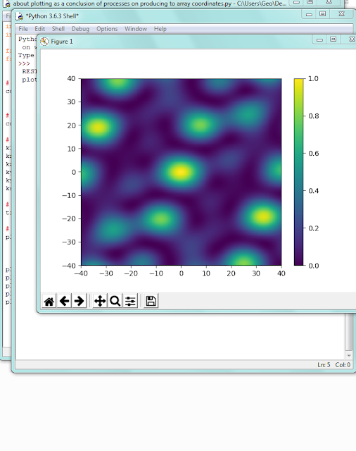
Where,shortly that
Coordinating in km via GENERATING OF ARRAY COORDINATES,next,setting to limits on analysis for wavenumber differences and finally compute transfer function as a function of wavenumber difference&plotting
By the way,for colour determination chapter;

And,a SlidePlayer presentation link on Array Response Functions
https://slideplayer.com/slide/6856804/
Some preprocessing studies on site array studies are my subject.In this context,last plot output that among considered distributions for carrying-out to array coordinates...
Site array studies which with having to big role into seismologic studies thus,role of technic a document about how tackling as a whole of Obspy will be quite important.
Yes...carrying-out to shortly "Site Array Determination"analysis at Site Check/Ispection Studies is requiring.Otherwise,among some possibilities for conclusions at site application;
So,You will evaluate that this analysis as a type optimisation step have to quite important role
New vision that shortly,expressing as "Synergy"
With this aim,widening of organisational structure is basepoint.For this,emphasizing to powerfulness of a "mass approach" on observing of European Hinterland on opensource programming language
As a conclusion of efforts in this field,a "Data Network Structure System" on Obspy&Python Programming Capabilities have developed.
Shortly,reading on internet network of basedata &carrying-out by user of some data process steps.And next,presenting on some types of some conclusions...
So,summarying as "Platform Structure"
On earthquake researches,providing to international a "synergy" on ground researches besides earthquake via user networks at hinterland countries for establishing as powerful of infrastructure can express.
I realised to some evaluations based on Obspy;
from obspy.core.util.base import get_example_file
from obspy.signal import PPSD
from obspy import read
from obspy.imaging.cm import pqlx
from obspy.io.xseed import Parser
from obspy.imaging.cm import viridis as cmap
from obspy.imaging.cm import _colormap_plot_array_response as plot
ppsd = PPSD.load_npz(get_example_file('ppsd_kw1_ehz.npz'))
ppsd.plot_temporal([0.1, 1, 10])
ppsd.plot("C:/users/Geo/Desktop/myprocessfile/ppsd.png")
ppsd.plot("C:/users/Geo/Desktop/myprocessfile/ppsd.pdf")
st = read("https://examples.obspy.org/BW.KW1..EHZ.D.2011.037")
parser = Parser("https://examples.obspy.org/dataless.seed.BW_KW1")
ppsd = PPSD(st[0].stats, metadata=parser)
ppsd.add(st)
ppsd.plot()
st = read("https://examples.obspy.org/BW.KW1..EHZ.D.2011.038")
ppsd.add(st)
ppsd.plot()
st = read("https://examples.obspy.org/BW.KW1..EHZ.D.2011.037")
parser = Parser("https://examples.obspy.org/dataless.seed.BW_KW1")
ppsd = PPSD(st[0].stats, metadata=parser)
ppsd.add(st)
st = read("https://examples.obspy.org/BW.KW1..EHZ.D.2011.038")
ppsd.add(st)
ppsd.plot(cmap=pqlx)
st = read("https://examples.obspy.org/BW.KW1..EHZ.D.2011.037")
parser = Parser("https://examples.obspy.org/dataless.seed.BW_KW1")
ppsd = PPSD(st[0].stats, metadata=parser)
ppsd.add(st)
st = read("https://examples.obspy.org/BW.KW1..EHZ.D.2011.038")
ppsd.add(st)
ppsd.plot(cumulative=True)
ppsd = PPSD.load_npz(get_example_file('ppsd_kw1_ehz.npz'))
ppsd.plot_spectrogram()
- Visualising probabilistic power spectral densities


A

B
Other presentation examples of 47/47 and 93/93 segments(A and B) for your data analysis studies

Amplitude-Period example of 93/93 Segment for your Data Analysis Studies

Amplitude-Period example as non-exceedance as cumulative of 93/93 Segment for your Data Analysis Studies

Amplitude Spectogram on Period-Time
- Time Frequency Misfit
from obspy.signal.tf_misfit import plot_tfr
import matplotlib.pyplot as plt
# general constants
tmax = 6.
dt = 0.01
npts = int(tmax / dt + 1)
t = np.linspace(0., tmax, npts)
fmin = .5
fmax = 10
# constants for the signal
A1 = 4.
t1 = 2.
f1 = 2.
phi1 = 0.
# generate the signal
H1 = (np.sign(t - t1) + 1) / 2
st1 = A1 * (t - t1) * np.exp(-2 * (t - t1))
st1 *= np.cos(2. * np.pi * f1 * (t - t1) + phi1 * np.pi) * H1
plot_tfr(st1, dt=dt, fmin=fmin, fmax=fmax)
from scipy.signal import hilbert
from obspy.signal.tf_misfit import plot_tf_misfits
# amplitude and phase error
phase_shift = 0.1
amp_fac = 1.1
# reference signal
st2 = st1.copy()
# generate analytical signal (hilbert transform) and add phase shift
st1p = hilbert(st1)
st1p = np.real(np.abs(st1p) * \
np.exp((np.angle(st1p) + phase_shift * np.pi) * 1j))
# signal with amplitude error
st1a = st1 * amp_fac
plot_tf_misfits(st1a, st2, dt=dt, fmin=fmin, fmax=fmax, show=False)
plot_tf_misfits(st1p, st2, dt=dt, fmin=fmin, fmax=fmax, show=False)
plt.show()from obspy.signal.tf_misfit import plot_tf_gofs
# amplitude and phase error
phase_shift = 0.8
amp_fac = 3.
# generate analytical signal (hilbert transform) and add phase shift
st1p = hilbert(st1)
st1p = np.real(np.abs(st1p) * \
np.exp((np.angle(st1p) + phase_shift * np.pi) * 1j))
# signal with amplitude error
st1a = st1 * amp_fac
plot_tf_gofs(st1a, st2, dt=dt, fmin=fmin, fmax=fmax, show=False)
plot_tf_gofs(st1p, st2, dt=dt, fmin=fmin, fmax=fmax, show=False)
plt.show()
# amplitude error
amp_fac = 1.1
# reference signals
st2_1 = st1.copy()
st2_2 = st1.copy() * 5.
st2 = np.c_[st2_1, st2_2].T
# signals with amplitude error
st1a = st2 * amp_fac
plot_tf_misfits(st1a, st2, dt=dt, fmin=fmin, fmax=fmax)
# amplitude and phase error
amp_fac = 1.1
ste = 0.001 * A1 * np.exp(- (10 * (t - 2. * t1)) ** 2) \# reference signal
st2 = st1.copy()
# signal with amplitude error + small additional pulse aftert 4 seconds
st1a = st1 * amp_fac + ste
plot_tf_misfits(st1a, st2, dt=dt, fmin=fmin, fmax=fmax, show=False)
plot_tf_misfits(st1a, st2, dt=dt, fmin=fmin, fmax=fmax, norm='local',
clim=0.15, show=False)
plt.show()


- Seismogram envelopes
import numpy as np
import matplotlib.pyplot as plt
import obspy
import obspy.signal
st = obspy.read("https://examples.obspy.org/RJOB_061005_072159.ehz.new")
data = st[0].data
npts = st[0].stats.npts
samprate = st[0].stats.sampling_rate
# Filtering the Stream object
st_filt = st.copy()
st_filt.filter('bandpass', freqmin=1, freqmax=3, corners=2, zerophase=True)
# Envelope of filtered data
data_envelope = obspy.signal.filter.envelope(st_filt[0].data)
# The plotting, plain matplotlib
t = np.arange(0, npts / samprate, 1 / samprate)
plt.plot(t, st_filt[0].data, 'k')
plt.plot(t, data_envelope, 'k:')
plt.title(st[0].stats.starttime)
plt.ylabel('Filtered Data w/ Envelope')
plt.xlabel('Time [s]')
plt.xlim(80, 90)
plt.show()

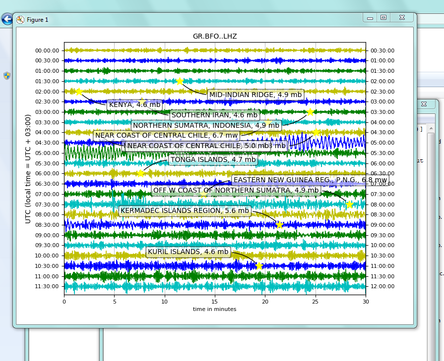
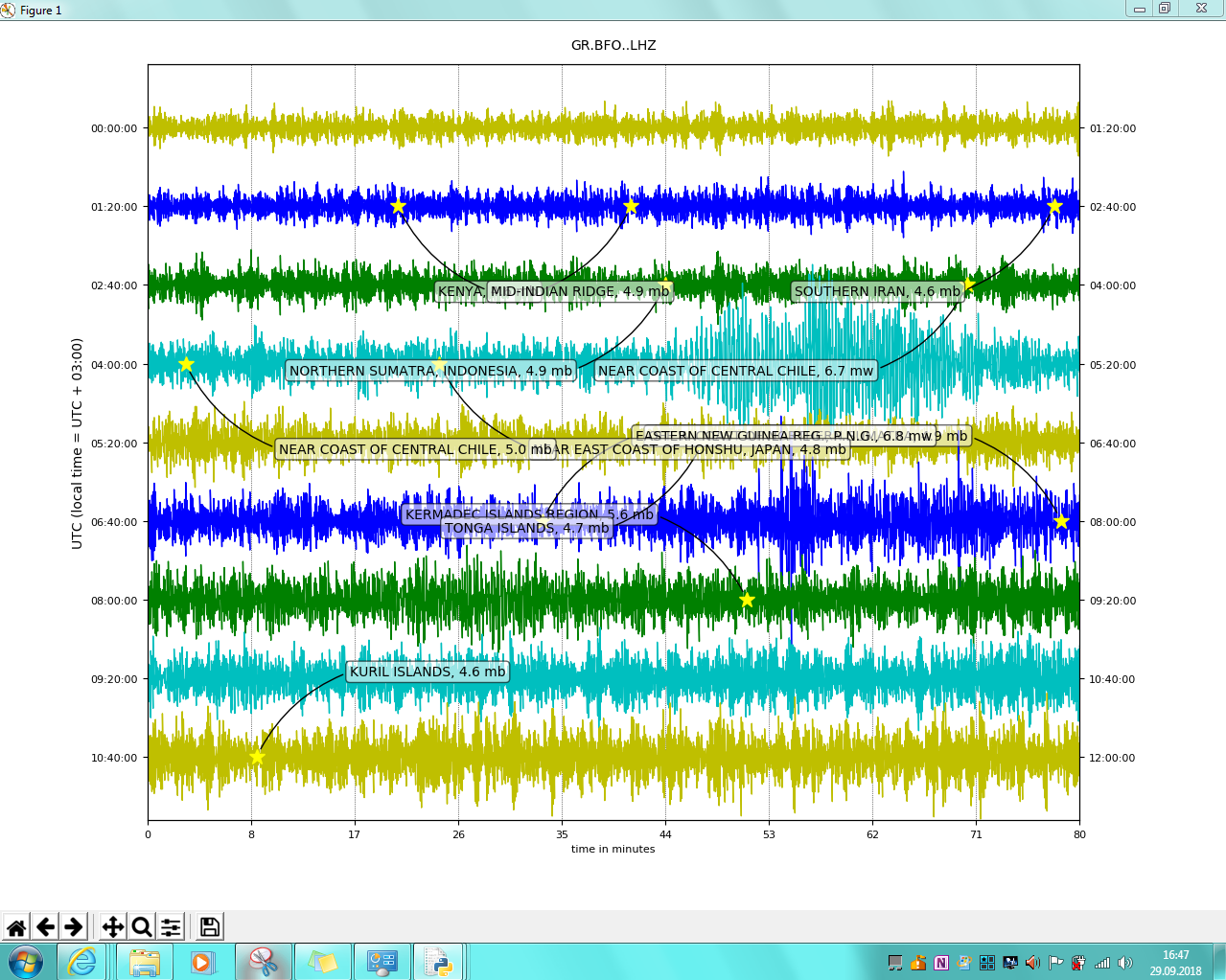
- Evaluating via multicode input on experimental features to Event Specifications
import obspy
st = obspy.read("https://examples.obspy.org/GR.BFO..LHZ.2012.108")
st.filter("highpass", freq=0.1, corners=2)
st.plot(type="dayplot", interval=30, right_vertical_labels=True,
vertical_scaling_range=5e3, one_tick_per_line=True,
color=['y', 'b', 'g', 'c'], show_y_UTC_label=True,
events={'min_magnitude': 4.0})
Example:
Interval=80
Interval=30
Magnitude Min=4.0
Conclusions of a working on events;
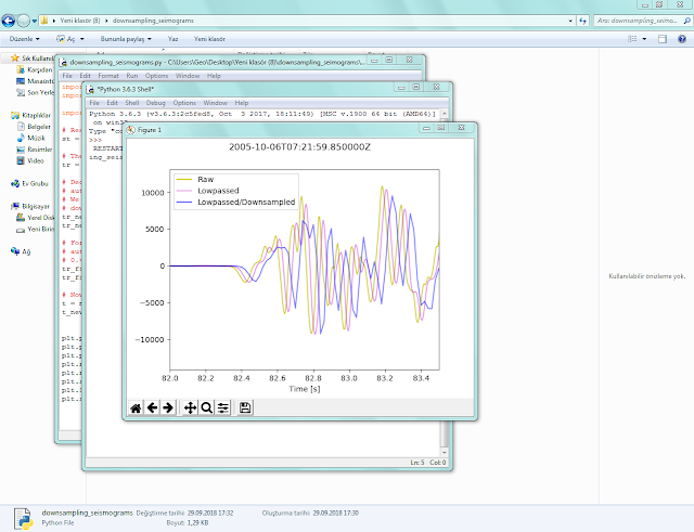
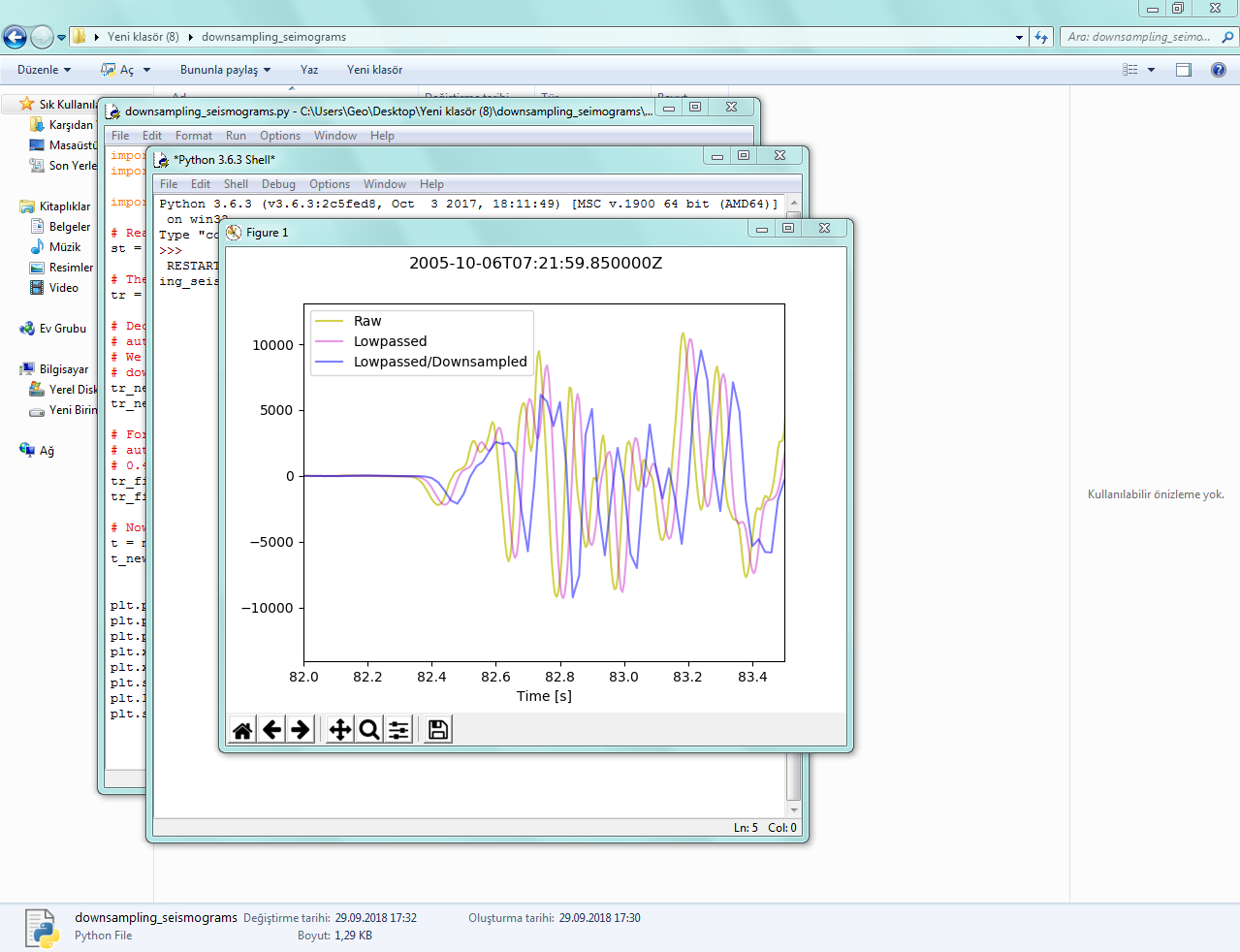
- Downsampling seismograms
import numpy as np
import matplotlib.pyplot as plt
import obspy# Read the seismogram
st = obspy.read("https://examples.obspy.org/RJOB_061005_072159.ehz.new")
# There is only one trace in the Stream object, let's work on that trace...
tr = st[0]
# Decimate the 200 Hz data by a factor of 4 to 50 Hz. Note that this
# automatically includes a lowpass filtering with corner frequency 20 Hz.
# We work on a copy of the original data just to demonstrate the effects of
# downsampling.
tr_new = tr.copy()
tr_new.decimate(factor=4, strict_length=False)
# For comparison also only filter the original data (same filter options as in
# automatically applied filtering during downsampling, corner frequency
# 0.4 * new sampling rate)
tr_filt = tr.copy()
tr_filt.filter('lowpass', freq=0.4 * tr.stats.sampling_rate / 4.0)
# Now let's plot the raw and filtered data...
t = np.arange(0, tr.stats.npts / tr.stats.sampling_rate, tr.stats.delta)
t_new = np.arange(0, tr_new.stats.npts / tr_new.stats.sampling_rate,
tr_new.stats.delta)
plt.plot(t, tr.data, 'y', label='Raw', alpha=0.7)
plt.plot(t, tr_filt.data, 'm', label='Lowpassed', alpha=0.4)
plt.plot(t_new, tr_new.data, 'b', label='Lowpassed/Downsampled', alpha=0.5)
plt.xlabel('Time [s]')
plt.xlim(82, 83.5)
plt.suptitle(tr.stats.starttime)
plt.legend()
plt.show()
- Continuous Wavelet Transform via Obspy
import matplotlib.pyplot as plt
import obspy
from obspy.imaging.cm import obspy_sequential
from obspy.signal.tf_misfit import cwt
st = obspy.read()
tr = st[0]
npts = tr.stats.npts
dt = tr.stats.delta
t = np.linspace(0, dt * npts, npts)
f_min = 1
f_max = 50
scalogram = cwt(tr.data, dt, 8, f_min, f_max)
fig = plt.figure()
ax = fig.add_subplot(111)
x, y = np.meshgrid(
t,
np.logspace(np.log10(f_min), np.log10(f_max), scalogram.shape[0]))
ax.pcolormesh(x, y, np.abs(scalogram), cmap=obspy_sequential)
ax.set_xlabel("Time after %s [s]" % tr.stats.starttime)
ax.set_ylabel("Frequency [Hz]")
ax.set_yscale('log')
ax.set_ylim(f_min, f_max)
plt.show()
Presentation-Conclusion on Obspy
import numpy as np
import matplotlib.pyplot as plt
import mlpy
import obspy
from obspy.imaging.cm import
obspy_sequential
wavelet_fct = "morlet"
scales = mlpy.wavelet.autoscales(N=len(tr.data), dt=tr.stats.delta,
dj=0.05,
wf=wavelet_fct,
p=omega0)
spec = mlpy.wavelet.cwt(tr.data, dt=tr.stats.delta, scales=scales,
wf=wavelet_fct, p=omega0)
# approximate scales through frequencies
freq = (omega0 + np.sqrt(2.0 + omega0 ** 2)) / (4 * np.pi *
scales[1:])
ax1 = fig.add_axes([0.1, 0.75, 0.7, 0.2])
ax2 = fig.add_axes([0.1, 0.1, 0.7, 0.60], sharex=ax1)
ax3 = fig.add_axes([0.83, 0.1, 0.03, 0.6])
t = np.arange(tr.stats.npts) / tr.stats.sampling_rate
ax1.plot(t, tr.data, 'k')
img = ax2.imshow(np.abs(spec), extent=[t[0], t[-1], freq[-1],
freq[0]],
aspect='auto', interpolation='nearest', cmap=obspy_sequential)
# Hackish way to overlay a logarithmic scale over a
linearly scaled image.
twin_ax = ax2.twinx()
twin_ax.set_yscale('log')
twin_ax.set_xlim(t[0], t[-1])
twin_ax.set_ylim(freq[-1], freq[0])
ax2.tick_params(which='both', labelleft=False, left=False)
twin_ax.tick_params(which='both', labelleft=True, left=True,
labelright=False)
fig.colorbar(img, cax=ax3)
plt.show()

Presentation-Conclusion on Machine Learning Module for Predictive Modelling
- Beamforming - FK Analysis
import matplotlib.pyplot as plt
import matplotlib.dates as mdates
import obspy
from obspy.core.util import AttribDict
from obspy.imaging.cm import obspy_sequential
from obspy.signal.invsim import corn_freq_2_paz
from obspy.signal.array_analysis import array_processing
# Load data
st = obspy.read("https://examples.obspy.org/agfa.mseed")
# Set PAZ and coordinates for all 5 channels
st[0].stats.paz = AttribDict({
'poles': [(-0.03736 - 0.03617j), (-0.03736 + 0.03617j)],
'zeros': [0j, 0j],
'sensitivity': 205479446.68601453,
'gain': 1.0})
st[0].stats.coordinates = AttribDict({
'latitude': 48.108589,
'elevation': 0.450000,
'longitude': 11.582967})
st[1].stats.paz = AttribDict({
'poles': [(-0.03736 - 0.03617j), (-0.03736 + 0.03617j)],
'zeros': [0j, 0j],
'sensitivity': 205479446.68601453,
'gain': 1.0})
st[1].stats.coordinates = AttribDict({
'latitude': 48.108192,
'elevation': 0.450000,
'longitude': 11.583120})
st[2].stats.paz = AttribDict({
'poles': [(-0.03736 - 0.03617j), (-0.03736 + 0.03617j)],
'zeros': [0j, 0j],
'sensitivity': 250000000.0,
'gain': 1.0})
st[2].stats.coordinates = AttribDict({
'latitude': 48.108692,
'elevation': 0.450000,
'longitude': 11.583414})
st[3].stats.paz = AttribDict({
'poles': [(-4.39823 + 4.48709j), (-4.39823 - 4.48709j)],
'zeros': [0j, 0j],
'sensitivity': 222222228.10910088,
'gain': 1.0})
st[3].stats.coordinates = AttribDict({
'latitude': 48.108456,
'elevation': 0.450000,
'longitude': 11.583049})
st[4].stats.paz = AttribDict({
'poles': [(-4.39823 + 4.48709j), (-4.39823 - 4.48709j), (-2.105 + 0j)],
'zeros': [0j, 0j, 0j],
'sensitivity': 222222228.10910088,
'gain': 1.0})
st[4].stats.coordinates = AttribDict({
'latitude': 48.108730,
'elevation': 0.450000,
'longitude': 11.583157})
# Instrument correction to 1Hz corner frequency
paz1hz = corn_freq_2_paz(1.0, damp=0.707)
st.simulate(paz_remove='self', paz_simulate=paz1hz)
# Execute array_processing
stime = obspy.UTCDateTime("20080217110515")
etime = obspy.UTCDateTime("20080217110545")
kwargs = dict(
# slowness grid: X min, X max, Y min, Y max, Slow Step
sll_x=-3.0, slm_x=3.0, sll_y=-3.0, slm_y=3.0, sl_s=0.03,
# sliding window properties
win_len=1.0, win_frac=0.05,
# frequency properties
frqlow=1.0, frqhigh=8.0, prewhiten=0,
# restrict output
semb_thres=-1e9, vel_thres=-1e9, timestamp='mlabday',
stime=stime, etime=etime
)
out = array_processing(st, **kwargs)
# Plot
labels = ['rel.power', 'abs.power', 'baz', 'slow']
xlocator = mdates.AutoDateLocator()
fig = plt.figure()
for i, lab in enumerate(labels):
ax = fig.add_subplot(4, 1, i + 1)
ax.scatter(out[:, 0], out[:, i + 1], c=out[:, 1], alpha=0.6,
edgecolors='none', cmap=obspy_sequential)
ax.set_ylabel(lab)
ax.set_xlim(out[0, 0], out[-1, 0])
ax.set_ylim(out[:, i + 1].min(), out[:, i + 1].max())
ax.xaxis.set_major_locator(xlocator)
ax.xaxis.set_major_formatter(mdates.AutoDateFormatter(xlocator))
fig.suptitle('AGFA skyscraper blasting in Munich %s' % (
stime.strftime('%Y-%m-%d'), ))
fig.autofmt_xdate()
fig.subplots_adjust(left=0.15, top=0.95, right=0.95, bottom=0.2, hspace=0)
plt.show()
import numpy as np
import matplotlib.pyplot as plt
from matplotlib.colorbar import ColorbarBase
from matplotlib.colors import Normalize
import obspy
from obspy.core.util import AttribDict
from obspy.imaging.cm import obspy_sequential
from obspy.signal.invsim import corn_freq_2_paz
from obspy.signal.array_analysis import array_processing
# Load data
st = obspy.read("https://examples.obspy.org/agfa.mseed")
# Set PAZ and coordinates for all 5 channels
st[0].stats.paz = AttribDict({
'poles': [(-0.03736 - 0.03617j), (-0.03736 + 0.03617j)],
'zeros': [0j, 0j],
'sensitivity': 205479446.68601453,
'gain': 1.0})
st[0].stats.coordinates = AttribDict({
'latitude': 48.108589,
'elevation': 0.450000,
'longitude': 11.582967})
st[1].stats.paz = AttribDict({
'poles': [(-0.03736 - 0.03617j), (-0.03736 + 0.03617j)],
'zeros': [0j, 0j],
'sensitivity': 205479446.68601453,
'gain': 1.0})
st[1].stats.coordinates = AttribDict({
'latitude': 48.108192,
'elevation': 0.450000,
'longitude': 11.583120})
st[2].stats.paz = AttribDict({
'poles': [(-0.03736 - 0.03617j), (-0.03736 + 0.03617j)],
'zeros': [0j, 0j],
'sensitivity': 250000000.0,
'gain': 1.0})
st[2].stats.coordinates = AttribDict({
'latitude': 48.108692,
'elevation': 0.450000,
'longitude': 11.583414})
st[3].stats.paz = AttribDict({
'poles': [(-4.39823 + 4.48709j), (-4.39823 - 4.48709j)],
'zeros': [0j, 0j],
'sensitivity': 222222228.10910088,
'gain': 1.0})
st[3].stats.coordinates = AttribDict({
'latitude': 48.108456,
'elevation': 0.450000,
'longitude': 11.583049})
st[4].stats.paz = AttribDict({
'poles': [(-4.39823 + 4.48709j), (-4.39823 - 4.48709j), (-2.105 + 0j)],
'zeros': [0j, 0j, 0j],
'sensitivity': 222222228.10910088,
'gain': 1.0})
st[4].stats.coordinates = AttribDict({
'latitude': 48.108730,
'elevation': 0.450000,
'longitude': 11.583157})
# Instrument correction to 1Hz corner frequency
paz1hz = corn_freq_2_paz(1.0, damp=0.707)
st.simulate(paz_remove='self', paz_simulate=paz1hz)
# Execute array_processing
kwargs = dict(
# slowness grid: X min, X max, Y min, Y max, Slow Step
sll_x=-3.0, slm_x=3.0, sll_y=-3.0, slm_y=3.0, sl_s=0.03,
# sliding window properties
win_len=1.0, win_frac=0.05,
# frequency properties
frqlow=1.0, frqhigh=8.0, prewhiten=0,
# restrict output
semb_thres=-1e9, vel_thres=-1e9,
stime=obspy.UTCDateTime("20080217110515"),
etime=obspy.UTCDateTime("20080217110545")
)
out = array_processing(st, **kwargs)
# Plotcmap = obspy_sequential
# make output human readable, adjust backazimuth to values between 0 and 360
t, rel_power, abs_power, baz, slow = out.T
baz[baz < 0.0] += 360
# choose number of fractions in plot (desirably 360 degree/N is an integer!)
N = 36
N2 = 30
abins = np.arange(N + 1) * 360. / N
sbins = np.linspace(0, 3, N2 + 1)
# sum rel power in bins given by abins and sbins
hist, baz_edges, sl_edges = \
np.histogram2d(baz, slow, bins=[abins, sbins], weights=rel_power)
# transform to radian
baz_edges = np.radians(baz_edges)
# add polar and colorbar axes
fig = plt.figure(figsize=(8, 8))
cax = fig.add_axes([0.85, 0.2, 0.05, 0.5])
ax = fig.add_axes([0.10, 0.1, 0.70, 0.7], polar=True)
ax.set_theta_direction(-1)
ax.set_theta_zero_location("N")
dh = abs(sl_edges[1] - sl_edges[0])
dw = abs(baz_edges[1] - baz_edges[0])
# circle through backazimuth
for i, row in enumerate(hist):
bars = ax.bar(left=(i * dw) * np.ones(N2),
height=dh * np.ones(N2),
width=dw, bottom=dh * np.arange(N2),
color=cmap(row / hist.max()))
ax.set_xticks(np.linspace(0, 2 * np.pi, 4, endpoint=False))
ax.set_xticklabels(['N', 'E', 'S', 'W'])
# set slowness limits
ax.set_ylim(0, 3)
[i.set_color('grey') for i in ax.get_yticklabels()]
ColorbarBase(cax, cmap=cmap,
norm=Normalize(vmin=hist.min(), vmax=hist.max()))
plt.show()


- some Obspy presentations on user capabilities
*Curves as Time(mimutes)-Distance(degree) of P-PP-S
from obspy.taup import plot_travel_times
import matplotlib.pyplot as plt
fig, ax = plt.subplots()
ax = plot_travel_times(source_depth=10, ax=ax, fig=fig,
phase_list=['P', 'PP', 'S'], npoints=200)

*Depth(km)-Distance(degree) Modelling as Sectional
from obspy.taup import TauPyModel
model = TauPyModel(model='iasp91')
arrivals = model.get_ray_paths(500, 140, phase_list=['PP', 'SSS'])
arrivals.plot_rays(plot_type='cartesian', phase_list=['PP', 'SSS'],
plot_all=False, legend=True)

*Pfdiff&SS Modelling Example on Earth Section
from obspy.taup import TauPyModel
model = TauPyModel(model='iasp91')
arrivals = model.get_ray_paths(500, 140, phase_list=['Pdiff', 'SS'])
arrivals.plot_rays(plot_type='spherical', phase_list=['Pdiff', 'SS'],
legend=True)

*Phase Distances
import numpy as np
import matplotlib.pyplot as plt
from obspy.taup import TauPyModel
PHASES = [
# Phase, distance
('P', 26),
('PP', 60),
('PPP', 94),
('PPS', 155),
('p', 3),
('pPcP', 100),
('PKIKP', 170),
('PKJKP', 194),
('S', 65),
('SP', 85),
('SS', 134.5),
('SSS', 204),
('p', -10),
('pP', -37.5),
('s', -3),
('sP', -49),
('ScS', -44),
('SKS', -82),
('SKKS', -120),
]
model = TauPyModel(model='iasp91')
fig, ax = plt.subplots(subplot_kw=dict(polar=True))
# Plot all pre-determined phases
for phase, distance in PHASES:
arrivals = model.get_ray_paths(700, distance, phase_list=[phase])
ax = arrivals.plot_rays(plot_type='spherical',
legend=False, label_arrivals=True,
plot_all=True,
show=False, ax=ax)
# Annotate regions
ax.text(0, 0, 'Solid\ninner\ncore',
horizontalalignment='center', verticalalignment='center',
bbox=dict(facecolor='white', edgecolor='none', alpha=0.7))
ocr = (model.model.radius_of_planet -
(model.model.s_mod.v_mod.iocb_depth +
model.model.s_mod.v_mod.cmb_depth) / 2)
ax.text(np.deg2rad(180), ocr, 'Fluid outer core',
horizontalalignment='center',
bbox=dict(facecolor='white', edgecolor='none', alpha=0.7))
mr = model.model.radius_of_planet - model.model.s_mod.v_mod.cmb_depth / 2
ax.text(np.deg2rad(180), mr, 'Solid mantle',
horizontalalignment='center',
bbox=dict(facecolor='white', edgecolor='none', alpha=0.7))
plt.show()

*Raypath Modelling Example of P&PKP Phases
from obspy.taup.tau import plot_ray_paths
import matplotlib.pyplot as plt
fig, ax = plt.subplots(subplot_kw=dict(polar=True))
ax = plot_ray_paths(source_depth=100, ax=ax, fig=fig, phase_list=['P', 'PKP'],
npoints=25)
**about plotting as a conclusion of processes on producing to array coordinates
import numpy as np
import matplotlib.pyplot as plt
from obspy.imaging.cm import obspy_sequential
from obspy.signal.array_analysis import array_transff_wavenumber
# generate array coordinates
coords = np.array([[10., 60., 0.], [200., 50., 0.], [-120., 170., 0.],
[-100., -150., 0.], [30., -220., 0.]])
# coordinates in km
coords /= 1000.
# set limits for wavenumber differences to analyze
klim = 40.
kxmin = -klim
kxmax = klim
kymin = -klim
kymax = klim
kstep = klim / 100.
# compute transfer function as a function of wavenumber difference
transff = array_transff_wavenumber(coords, klim, kstep, coordsys='xy')
# plot
plt.pcolor(np.arange(kxmin, kxmax + kstep * 1.1, kstep) - kstep / 2.,
np.arange(kymin, kymax + kstep * 1.1, kstep) - kstep / 2.,
transff.T, cmap=obspy_sequential)
plt.colorbar()
plt.clim(vmin=0., vmax=1.)
plt.xlim(kxmin, kxmax)
plt.ylim(kymin, kymax)
plt.show()

Where,shortly that
Coordinating in km via GENERATING OF ARRAY COORDINATES,next,setting to limits on analysis for wavenumber differences and finally compute transfer function as a function of wavenumber difference&plotting
By the way,for colour determination chapter;

And,a SlidePlayer presentation link on Array Response Functions
https://slideplayer.com/slide/6856804/
Some preprocessing studies on site array studies are my subject.In this context,last plot output that among considered distributions for carrying-out to array coordinates...
Site array studies which with having to big role into seismologic studies thus,role of technic a document about how tackling as a whole of Obspy will be quite important.
Yes...carrying-out to shortly "Site Array Determination"analysis at Site Check/Ispection Studies is requiring.Otherwise,among some possibilities for conclusions at site application;
- Disadvantages as Time-consuming and extraeffort due to excessive data collecting
- Problems of caused data quality of Data Deficient
So,You will evaluate that this analysis as a type optimisation step have to quite important role

Yorumlar
Yorum Gönder